Download
1 / 32
320 likes | 417 Views
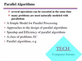
Paradigms for Parallel Algorithms. Levels of Parallelism. (Sub)Program Level Parallelism. Program Level Parallelism If there are n independent programs, these programs can be given to n different processing elements (or machines).

E N D
Paradigms for Parallel Algorithms Paradigms for Parallel Algorithms
Levels of Parallelism Paradigms for Parallel Algorithms
(Sub)Program Level Parallelism Program Level Parallelism • If there are n independent programs, these programs can be given to n different processing elements (or machines). • Since programs are implemented in parallel, this is a high-level parallelism. Subprogram Level Parallelism • A program can be divided into smaller subprograms. • These subprograms can be executed in parallel. Paradigms for Parallel Algorithms
Statement Level Parallelism • In any program (or subprogram) there are several statements. These statements may be done in parallel. • For example: For i = 1 to n do xi = xi + 1; This statement is repeated n times sequentially and O(n) time is needed. This can be parallelized by n processors simultaneously in O(1) time. For i = 1 to n do in parallel xi = xi + 1; End-parallel Paradigms for Parallel Algorithms
S = + + + + + + … … x1x2 x3x4 xn-1xn Operation Level Parallelism • In a statement, several operations are carried out. We can think of parallelizing these operations. • For example: S = x1 + x2 + … + xn This cannot be parallelized as the case in statement level parallelism. It can be parallelized by using n/2 processors, to work in O(log n) time. Paradigms for Parallel Algorithms
Micro Operation Level Parallelism • Usually, any operation consists of several micro-operations. These operations may be done in parallel. • For example: C = A + B; There are three micro-operations. • Load the accumulator with the content of A. • Add the content of B with the content of the accumulator. • Store the content of the accumulator in the variable C. Paradigms for Parallel Algorithms
PRAM Model • In the PRAM (Parallel Random Access Machine) model, all the processors are connected in parallel to a global large memory. • This is also called a shared-memory model. • All the processors are assumed to work synchronously on a common clock. • Depending upon the capability of more than one processors to read from/write to a memory location, there are four different types: EREW, CREW, ERCW, and CRCW. Paradigms for Parallel Algorithms
Four Types of PRAM • EREW (Exclusive Read Exclusive Write PRAM): • It permits only one processor at one instant to read from/write to a memory location. • Simultaneous reading or simultaneous writing by more than one processors in a memory location is not permitted here. • CREW (Concurrent Read Exclusive Write PRAM): • It permits concurrent reading of a location by more than one processor, but does not permit concurrent writing. • ERCW (Exclusive Read Concurrent Write PRAM): • It permits concurrent writing alone. Paradigms for Parallel Algorithms
Four Types of PRAM • CRCW (Concurrent Read Concurrent Write PRAM): • It is the most powerful model, which permits concurrent reading, as well as concurrent writing in a memory location. • When one or more processors tries to read the content of a memory location concurrently, we assume that all those processors succeed in reading. • However, when more than one processors try to write to the same location concurrently, the conflict has to be properly resolved. Paradigms for Parallel Algorithms
Methods of Resolving Conflict • ECR (Equality Conflict Resolution): The processors succeed in writing, only if all the processors try to write the same value to the location. • PCR (Priority Conflict Resolution): Each processor has its priority number. When more than one processors try to write to the same location simultaneously, the processor with highest priority succeeds. • ACR (Arbitrary Conflict Resolution): Among the processors trying to write simultaneously, some arbitrary processor succeeds. Paradigms for Parallel Algorithms
Sequential Algorithm of Boolean-AND Example: RESULT = A(1) A(2) A(3) … A(n) Algorithm Sequential-Boolean-AND Input: The Boolean array A(1:n) Output: The Boolean value RESULT BEGIN RESULT = TRUE; For i = 1 to n do RESULT = RESULT A(i); End-For END. O(n) time with O(1) PE Paradigms for Parallel Algorithms
Parallel Alg. for ERCW-ACR Model Algorithm Parallel-Boolean-AND-ACR Input: The Boolean array A(1:n) Output: The Boolean value RESULT BEGIN RESULT = TRUE; For i = 1 to n do in parallel If A(i) = FALSE then RESULT = FALSE; End-If End-parallel END. *It’s also suited for ERCW-PCR & ECR model. O(1) time with O(n) PEs Paradigms for Parallel Algorithms
Parallel Alg. for ERCW-ECR Model Algorithm Parallel-Boolean-AND-ECR Input: The Boolean Array A(1:n) Output: The Boolean value RESULT BEGIN RESULT = FALSE; For i = 1 to n do in parallel RESULT = A(i); End-parallel END. O(1) time with O(n) PEs Paradigms for Parallel Algorithms
Parallel Processing for EREW Model • The elementary AND operation is a binary operation. When n is the size of the data, the AND operation can be performed by the n/2 processors simultaneously. • Processor Pi does A(i) A(2i – 1) A(2i). Ex: P1 : A(1) A(2) P2 : A(3) A(4) … Pn/2 : A(n-1) A(n) Paradigms for Parallel Algorithms
Stage (log n) ^ ^ ^ ^ ^ ^ … Stage 1 … A(1) A(2) A(3) A(4) A(n-1) A(n) Parallel Processing for EREW Model • After the first stage, there are n/2 results which can be used as data for next iteration. • In the second stage, only n/4 processors are needed for n/2 of data. • All processing can be done in O(log n) stages. Paradigms for Parallel Algorithms
Parallel Alg. for EREW Model Algorithm Parallel-Boolean-AND-EREW Input: The Boolean Array A(1:n); Number of PEs p Output: The Boolean value RESULT BEGIN p = n / 2; While p > 0 do For i = 1 to p do in parallel A(i) = A(2i – 1) A(2i); End-parallel p = p/2; End-While RESULT = A(1); END. O(log n) time with O(n) PEs Paradigms for Parallel Algorithms
Binary Tree Paradigm Sum of n Numbers: Consider the problem of summation of n numbers. It takes O(n) time for a single processor to sum n numbers. • Assume that n = 2k = 8 and there are n/2 (= 4) processors. Suppose the sample data as shown below: Paradigms for Parallel Algorithms
Parallel Algorithm for Sum Algorithm Parallel-SUM Input: Array A(1:n) where n=2k. Output: The sum of the values of the array stored in A(1). BEGIN p = n / 2; While p > 0 do For i = 1 to p do in parallel A(i) = A(2i – 1) + A(2i); End-parallel p = p/2; End-While END. Paradigms for Parallel Algorithms
Parallel Processing of Sum 1st stage: P1 do A(1) A(1) + A(2) = 68 P2 do A(2) A(3) + A(4) = 76 P3 do A(3) A(5) + A(6) = 96 P4 do A(4) A(7) + A(8) = 73 2nd stage: P1 do A(1) A(1) + A(2) = 144 P2 do A(2) A(3) + A(4) = 169 3rd stage: P1 do A(1) A(1) + A(2) = 313 Paradigms for Parallel Algorithms
Complexity Analysis • The algorithm doesn’t use concurrent reading or concurrent writing anywhere. • This can be done by O(log n) time with O(n) PEs in EREW PRAM model. Paradigms for Parallel Algorithms
Pointer Jumping List Ranking Problem: Let A(1:n) be an array of numbers. They are in a linked list in some order. The rank of the number is defined to be its distance from the end of the linked list. • The last number in the linked list has the rank 1 and the next one has rank 2, and so on. The first entry of the linked list is of rank n. • The variable HEAD contains the index of the first number. • Let LINK(i) denote the index of the number next to A(i). Ex. LINK(3) = 7 means that in the linked list A(7) is the number next to A(3). LINK(i) = 0 if A(i) is the last entry in the linked list. Paradigms for Parallel Algorithms
A(5) 0 270 HEAD A(1) A(7) A(4) A(3) A(2) A(6) A(8) 187 93 43 215 192 21 201 Example of List Ranking Paradigms for Parallel Algorithms
Sequential Algorithm of List Ranging Algorithm Sequential-List-Ranging Input:A(1:n), LINK(1:n), HEAD Output:RANK(1:n) BEGIN p = HEAD; r = n; RANK(p) = r; Repeat p = LINK(p); r = r – 1; RANK(p) = r; Until LINK(p) is equal to 0. END. Paradigms for Parallel Algorithms
Grow Doubling Variable • To develop the parallel algorithm, there is a new variable NEXT(i). • Initially NEXT(i) = LINK(i). That is, NEXT(i) initially denotes the index of its right neighbor. • At the next step we should have NEXT(i) = NEXT(NEXT(i)). Now NEXT(i) denotes the entry at distance 2. At next stage, NEXT(i) will be denote the entry at distance 4, that is , NEXT(i) grows by doubling. Paradigms for Parallel Algorithms
Parallel Algorithm of List Ranging Algorithm Parallel-List-Ranging Input:A(1:n), LINK(1:n), HEAD Output:RANK(1:n) BEGIN For i = 1 to n do in parallel RANK(i) = 1; NEXT(i) = LINK(i); End-parallel For k = 1 to (log n) do For i = 1 to n do in parallel If NEXT(i) 0 RANK(i) = RANK(i) + RANK(NEXT(i)); NEXT(i) = NEXT(NEXT(i)); End-If End-parallel End_For END. O(log n) time with O(n) PEs in CREW Paradigms for Parallel Algorithms
A(5) 0 21 HEAD A(1) A(7) A(4) A(3) A(2) A(6) A(8) 187 93 43 215 192 21 201 Parallel Processing of Initial Stage Paradigms for Parallel Algorithms
A(5) NEXT NEXT NEXT NEXT NEXT NEXT NEXT 0 270 HEAD A(3) A(7) A(1) A(8) A(2) A(6) A(4) 192 201 187 93 43 21 215 Parallel Processing of Stage 1 Paradigms for Parallel Algorithms
NEXT NEXT NEXT NEXT NEXT NEXT A(8) A(5) 0 0 215 270 HEAD A(3) A(7) A(1) A(6) A(2) A(4) 192 187 93 43 21 201 Parallel Processing of Stage 2 Paradigms for Parallel Algorithms
NEXT NEXT NEXT NEXT A(6) A(8) A(5) 0 0 0 201 215 270 HEAD A(7) A(2) A(3) A(1) A(4) 192 93 43 21 187 Parallel Processing of Stage 3 Paradigms for Parallel Algorithms
Divide and Conquer • The problem is divided into smaller subproblem. The solutions of these subproblems are processed further, to get the solution of the complete problem. • If A(1:n) is an array, the parallel algorithm for sum of the entries in O(log n) time by using O(n) PEs is not an optimal one. • The array of numbers A1, A2, …, An can be divided into r (= n/log n) groups, each containing (log n) entries. The following are the groups: Paradigms for Parallel Algorithms
Divide and Conquer Group 1: A1, A2, ………………….…………….., Alog n Group 2: Alog n +1, Alog n +2, …………..………….., A2log n Group 3: A2log n +1,A2log n +2, …………………….., A3log n … Group r: A(r-1)log n +1, A(r-1)log n +2, …..………..….., An • Let’s assign each group to one processor. So, there are n/(log n) processors needed. • Each processor Pi add (log n) elements sequentially and stores the result in variable Bi (1 i r). • Using thealgorithm Parallel-SUM to add these variables B1 to Br. Paradigms for Parallel Algorithms
Algorithm of Optimal Parallel Sum Algorithm Optimal-Parallel-SUM Input: Array A(1:n) where n=2k. Output: The sum of the values of the array stored in SUM. BEGIN For i = 1 to (n/log n) do in parallel Bi= A(i-1)log n + 1 + A(i-1)log n + 2 + … + Ailog n ; End-parallel SUM = Parallel-SUM(array B); END. O(log n) time with O(n/log n) PEs in EREW PRAM Paradigms for Parallel Algorithms