Download
1 / 75
760 likes | 835 Views
Explore the quantum treatment of electromagnetic radiation fields, including Maxwell's equations and the Casimir effect, through harmonic oscillator quantization techniques. Learn about coherent states and the bosonic nature of light.

E N D
Field Quantization Speaker: Yenon Benhaim
Outline • Introduction • Potential theory for the Classical E.M field. • Maxwell Eq – Derivation from Lagrangian • Quantum Harmonic Oscillator • Quantum treatment for light (quantization) • The Casimer effect • Coherent States • Beam-Splitter • Bosonic Nature of Light • Conclusion • Reference
Introduction: We know from Planckws law, that the energy of the radiation field are Quantized.
But most of the calculation of the EM radiation field are based on the semi-classical theory, in which the radiation fields E and B are treated as classical variables while the atoms are treated quantum-mechanically. A more consistent theory must treat the whole system of radiation and atoms in quantum-mechanical terms, with the fields represented by operators E and B. We will see that the quantization introduces characteristic Q.M effects into the properties of the radiation field. (uncertainty principles between E and B)
Potential theory for the Classical E.M field. The field vectors in QM must be taken as operators instead of the algebraic quantities of classical theory, but both theories based on the familiar Maxwell Equations.
Maxwell equations: Gauss’ Law Coulomb’s Law Faraday’s Law Ampere’s Law Where and J are the charge and current densities, respectively. The classical fields and densities are functions of position ant time
From the symmetry of the Maxwell Eq, it’s easy to see that the result for the Magnetic field will be of the form : Combine with our previous result for E: We can understand why we can treat the light as E.M – waves.
We can get Maxwell Eq by lagragiean formalism: By defining the F tensor to be: The Inhomogeneous Maxwell Eq Become: For Example :
The Homogenous Maxwell Eq : We can see that by working with our definition of F – we don’t need to worry about the homogenous part of Maxwell eq.
So the Maxwell Eq can be written in 2 forms (with are identical) : By substituting this equations we can get the wave behavior of light (E.M Waves)
We can define the Lagrangeian to be : The Oiler-Lagrange formula is : In our case : And we get the Maxwell Eq :
The quantization is facilitated if the classical Maxwell equation are re-expressed in terms of the scalar and vector potentials , and A : After substitution this eq in the classical Maxwell equation we get the field equations :
We can simplified this equation, by using the Coulumb gauge: Gauge Transformation Coulumb gauge: And we get:
We can separate each vector to longitudinal and transverse components (According to Helmholtz theorem) The same goes for the other field, B which is independent of gauge and depend only on AT we can see that After substituting we have a longitudinal and transverse equation :
The scalar potential satisfies: Which is the eq of charge conservation. The electric vector can also be divided into transverse and longitudinal parts: The magnetic vector B is entirely transverse according to the Maxwell
Thus we can write the Transverse part of Maxwall eq as : The transverse eq describe EM waves, which are influenced only by the transverse part of the current density.
The longitudinal Maxwell eq on the other hand are: The longitudinal equations describe the electric fields that arise from the charge density, as determined by the equations of electrostatics.
The Quantum Story • The central step in the quantization is the replacement of a classical harmonic oscillator by the corresponding QM harmonic oscillator. • The quantization of the E.M field proceeds by the replacement of the classical vector potential A, by Q.M operator A.
The Quantum Story Consider a cubic region of side L: The cavity is now regarded merely as a region of space without any real boundaries, known as the “quantization cavity”. We take running waves solutions of the field and subject them to periodic boundeary conditions. L
In free space (when J=0) we get : The solutions for the wave eq for A is : Where : - unit polarization vectors The coulomb gauge condition – requires that The polarization are chosen to be perpendicular to each other
Each mode components of the vector potential are independent and they separately obey the field equation : The mod coefficients, and their complex conjugates, thus satisfy the simple-harmonic equation of motion: The E.M field is quantized by conversion of the classical H.O to Q.M counterpart. The nature of the conversion is suggested by the form of the field energy, which we now evaluate.
The solution to the wave eq for A is taken the form : The mode contribution to the vector potential becomes : The complete vector potential is obtained by substitution of this expression into : The corresponding complete transverse electric field is obtained from :
And the magnetic field is obtained from: The total energy of the E.M radiation field in the cavity is : After some algebra – the total radiative energy reduces to a sum of time – independent contributions from the individual modes.
Quantum Harmonic Oscillator I would like to remind you of the way of solving the quantum harmonic oscillator. The Hamiltonian is in this case given by We can define the raising and lowering operators.
Writing back the Hamiltonian with this definitions : Also we can compute the commutator relations : The state |n> can be written as: Then the energies are :
We can count the number of excitation in the system as : The energy level is than quantized as:
Quantization of the E.M field • The E.M field is quantzed by the association of a Q.M harmonic oscillator with each mod kλ of the radiation field in the quantization cavity. • Thus the destruction and creation operator take the forms :
The operators destroy and create one photon of energy in mode . Note that the angular frequency of the photon depends only on the magnitude of its wavector and it is independent of the mode polarization specified by the index λ=2.3. The number of photons excited in the cavity mode is given by the eignvalue of the operator : With the eignvalue relation:
The orthonormal eigenstates ,|n> are known as the “photon-number state” or “Fock states” of the E.M field. A number state of the total E.M field in the cavity is specified by a string of photon numbers, one for each of the allowed modes. The different cavity modes are independent, and their associated operators commute : The state of the total field is written as a product of states of the individual modes: Denots the complete set of numbers that specify the excitation levels of all the H.O associated with the cavity modes. There are infintely many such oscillators. - which form a complete set of states for the E.M field.
The hamiltonian of the radiation field is obtaind by summation of the H.O contributions as: where Comparison with the expression we got earlier : And
With these substitutions, the classical vector potential is converted to the operator : where The expressions for the operators are simplified by defining a phase angle for the mode waveforms by
The complete electric – field operator is conveniently separated as: Where the two contributions are: And are known respectively as the “positive” and “negative frequency parts” of the E.M field operators. This names are somewhat counter-intuitive, as the plus sign is associated with the destruction operator components and the minus sign with the creation operator.
The magnetic field operator is written in the analogous form: Where This operators of the magnetic and electric fields are Hermitian, and they represent the observable E.M fields in the cavity. The E.M radiation Hamiltonian is written in a form analogous to the classical energy as
The energy is then The energy eigen-value relation for the multimode number state is: The ground state of the E.M filed in which no photons are excited in any of the filed modes, that is For all k and λ Is called the “vacuum state of the field. The vacuum state is denoted |0>, and it satisfies ground-state conditions of the form For all k and λ
The ground state energy is: Is known as the “zero – point energy” or “vacuum energy”. This contribution has no analogue in the classical theroy. The eignvalue relation can be written as Where Is the excitation enrgy of the E.M field above its zero – point value
Zero-point energy The state |{0}i, referred to as the vacuum state, is the state of lowest energy and corresponds to the state for which all the occupation numbers nk are zero. Although no excitations are present, the total energy does not vanish. The energy of this state is which is equal to infinity. It is the sum of the energies of the ground state of each harmonic oscillator and it is infinite because there is no upper bound to the field’s frequency.
There is no satisfactory explanation for the physical significance of this, but, fortunately, we can eliminate this term by shifting the energy of the ground state. This infinite energy shift can not be detected experimentally, since the experiments measure only energy differences from the ground state of HEM. This infinite constant term, called the zero point energy of the radiation field, is responsible for many interesting effects. Some phenomena which could not be explained using classical fields such as the Casimir effect.
Casimir Forces Casimir forces provide a straightforward illustration of vacuum effects. Suppose that a plane parallel cavity made from a pair of perfectly conducting and reflecting mirrors a distance L apart is placed in free space. We consider the change in the vacuum energy brought about by the presence of the cavity. The energy in the free space regions on both sides of the cavity remains the same but the energy inside the cavity is modifed by the change in mode structure from continuous to discrete. The vacumm energy of the standing wave modes with wavevector perpendicular to the mirrors is :
The vacuum energy in the same region of space in the absence of the cavity is given by the same expression but with the wavevector replaced by a continuous variable Both these expression for the vacuum energy are clearly infinite. Consider, however the change in energy produced by the presence of the cavity, given by the difference of these exprressions: It follows that the energy diminishes with decreeasing L, and there is an attractive force between the mirrors given by:
The force ia an example of the casimir forces that act between all bodies placed in the E.M vacuum. This calculation of the force between two parallel mirrors takes account only of the modes witg wavevectors perpendicular to the mirrors. Arealistic 3D theroy must include the contributios of all wavevector orientations. The principles of the calculation remain the same but the Casimir force per unit area, or pressure, is given by
MaritimeAnalogy There is an interesting maritime analogy with the Casimir effect that just shows clearly how the wave-like nature of particles is responsible for the some-what counter-intuitive vacuum effects. This is a real life story about the warning issued to sailors (this was a few centuries ago or so) that two ships which are docked in a harbour parallel to each other may start to approach each other (and may ultimately crash into each other) due to their small oscillations up and down in the water. The explanation of this effect, which is remarkably similar to the Casimir force, lies in the fact that the waves that exist between the two ships actually cancel each other out, while the waves going away from the ships don’t. This means that due to the conservation of momentum the ships recoil towards each other and this is the origin of the maritime force.
The force can even be calculated to be • where m is the mass of the ship, h its amplitude of oscillations, A the angle from the normal to the water surface and T the period of oscillations. • If m = 700 tons, h = 1.5 meters, A = 8 degrees T = 8 seconds • we obtain the force F = 102 Newtons, which is by no means a negligible force.
Proposed Experiment 40 μm diamater, 20 μm thick disk made out of quartz or calcite is placed on top of a BaTiO3 plate immersed in ethanol. For distances shorter than a few nanometers, the force is attractive. However, at larger distances, where retardation effects start to play an important role in the interaction, the force switches to repulsive.
it is possible to show that the force between two plates with dielectric functions έ1 and έ2 immersed in a medium with dielectric function έ3 is repulsive if, for imaginary frequencies, έ1,<έ3<έ2 or έ2< έ3<έ1, and it is attractive in all other cases . The force is thus repulsive at large distances
In this case the Casimir forces between the two birefringent slabs is repulsive. The disk is thus expected to float on top of the plate at a distance of approximately 100 nm, where its weight is counterbalanced by the Casimir repulsion. Because there is no contact between the two birefringent surfaces, the disk would be free to rotate in a sort of frictionless bearing, sensitive to even very small driving torques.
A 100 mW laser beam can be collimated onto the disk to rotate it by the transfer of angular momentum of light. A shutter can then block the beam to stop the light induced rotation. The position of the disk can be monitored by means of a microscope objective coupled to a CCD camera for imaging.
Using the laser, one can rotate the disk until . Once the laser beam is shuttered, the disk is free to rotate back towards the configuration of minimum energy according to the following equation where R is the radius of the disk, I is its momentum of inertia, ή is the viscosity of ethanol (1.2x10⁻³ Ns/m2) , d is the distance between the disk and the plate, and a sin(2θ) is the torque due to quantum fluctuations.
Note that the rotation is over-damped in both cases: the disk moves asymptotically and monotonically towards the equilibrium position. For the calcite disk, easily measurable rotations should be observed within a few minutes after the laser beam shutter is closed. The quartz disk would rotate much more slowly, and it is questionable whether its rotation could be detected or not.
Coherent States The multimode number states we defined earlier Form a complete set of basis states for the E.M field. A general pure state of the E.M field is expressible as superposition of these basis states, of the form The full generality of this state is rarely used, but there are important pure states of the radiation field in which the superposition is restricted to the number states of a single mode, for example the coherent states. Not all excitations of the radiation field are expressible as linear superposition of this basis.