Download
1 / 45
450 likes | 711 Views
Improvements to A-Priori. Bloom Filters Park-Chen-Yu Algorithm Multistage Algorithm Approximate Algorithms Compacting Results. http://infolab.stanford.edu/~ullman/mining/2009/index.html. Aside : 基于哈希的过滤. 问题 : 有一个集合 S ,有 10 亿字符串,每个字符串 10 个字节 . 扫描文件 F ,输出那些在集合 S 中的字符串 . 只有 1GB 的主内存 .

E N D
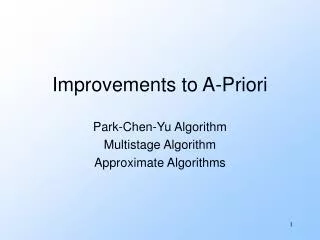
Improvements to A-Priori Bloom Filters Park-Chen-Yu Algorithm Multistage Algorithm Approximate Algorithms Compacting Results
Aside:基于哈希的过滤 • 问题: 有一个集合S,有10亿字符串,每个字符串 10个字节. • 扫描文件F,输出那些在集合S中的字符串. • 只有1GB 的主内存. • 无法把S存入主内存.
Solution – (1) • 建立一个 80亿比特的比特数组,初始化为0. • 选择一个哈西函数,输出范围 [0, 8*109), 把S中的每一个字串映射到该数组的一个位置上,并把该位置置为1.. • 哈西文件的每一个比特串,如果比特数组在该位置上值为1,则输出该比特。
输出; 可能在S. 为何不是必定? 丢弃;肯定不在S. Solution – (2) Filter File F h 0010001011000
Solution – (3) • 最多1/8 的比特数组的值为1,不在S中但是能够输出的字符串的概率最多是1/8. • 如果字符串在S,肯定哈西到值为1的位置,从而能够输出。. • 使用另外一个哈西函数和比特数组,降低虚警概率 • 降低1/ 8.
Aside: 扔飞镖 • 经常遇到飞镖问题: 如果把k个飞镖扔到n个等可能的目标, 一个目标至少命中一个飞镖的概率是多少? • Example: targets = bits, darts = hash values of elements. • 纯随机扔飞镖,命中的概率,也就是虚警概率
Equals 1/e as n ∞ Equivalent n( /n) k 1 - (1 – 1/n) 1 – e–k/n Probablity target not hit by one dart Probability at least one dart hits target Throwing Darts – (2)
Throwing Darts – (3) • 如果k << n, 则 e-k/n可以用两阶泰勒级数近似: 1 – k/n. • Example: 109 darts, 8*109 targets. • True value: 1 – e-1/8 = .1175. • Approximation: 1 – (1 – 1/8) = .125.
Improvement: Superimposed Codes (Bloom Filters) • 分别用两个哈西函数,把S的每一个元素映射到比特数组的两个比特. • 数组的 ¼ 是比特 1’s. • 只有两个比特位置都是1,才输出文件F的一个字符串,. • (1/4)2 = 1/16.
Superimposed Codes – (2) • 可以使用任意数目的哈西函数. • 哈西函数的数目越多,虚警概率反而变大. • Limiting Factor: 最后,比特数组所有比特都为1. • 所有字符串都哈西到 1’s.
Aside: History • The idea is attributed to Bloom (1970). • .
改进1:PCY Algorithm – An Application of Hash-Filtering • 在A-priori 的第一轮中,多数缓存是空闲的. • 使用这些缓存来存储项对哈希到的bucket的计数器. • 把一个项对哈西到一个计数器位置,可能有多个项对被哈西到同一个位置 • 只计数,不记录项对本身.
Needed Extensions to Hash-Filtering • 项对需要从输入文件中产生;项对本身不再文件中. • 不仅想知道是否存在一个项对,还想知道是否出现了s次 (支持度).
PCY Algorithm – (2) • 如果项对哈西到的桶的计数值至少是支持度门限,这个桶称为是频繁的。. • 如果一个项对哈西到的桶不是频繁的,桶内没有一个项对是频繁的。 • On Pass 2, 只计数那些在频繁桶内出现的项对.
Picture of PCY Hash table Item counts Frequent items Bitmap Counts of candidate pairs Pass 1 Pass 2
PCY Algorithm – Before Pass 1 Organize Main Memory • 每个项的计数器. • 每个项4个字节. • 剩余空间作为桶的计数器.
PCY Algorithm – Pass 1 FOR (each basket) { FOR (each item in the basket) add 1 to item’s count; FOR (each pair of items) { hash the pair to a bucket; add 1 to the count for that bucket } }
Observations About Buckets • 一个频繁项对哈西到的桶必定也是频繁的. • 计数器的值只增加不减少. • 即使没有频繁项对, 桶也可能是频繁的. • 多个项对被哈西到一个桶里. .
Observations – (2) 3.多数情况下, 桶的计数值小于支持度s. • 所有哈西到该桶的项对都不可能是频繁项对,尽管这个项对是由两个频繁项构成. • Thought question: 在什么情况下,我们现情况 3?
PCY Algorithm – Between Passes • 第一阶段扫描以后,用比特向量代替哈西计数器,以节约空间: • 1 表示桶是频繁的; 0 表示不是频繁的. • 四个字节的计数器值由比特替换,内存只是原来的 1/32. • 同时,还要保留频繁项列表.
PCY Algorithm – Pass 2 • 对满足下列条件的项对 {i, j } 计数: • i和j都是频繁项. • 项对 {i, j }哈西到的比特向量位置上的值为1. • 这两个条件是一个项对成为频繁项对的必要条件.
Memory Details • 每个Buckets需要几个字节. • Note: 如果计数值超过s,就不必增加了. • # buckets is O(main-memory size). • 在第二轮,a table of (item, item, count) triples is essential (why?). • PCY如果要优于a-priori,需要消除 2/3 的可能的项对.
改进2: Multistage Algorithm • Key idea: 经过了PCY的第一阶段,重新哈西那些满足PCY第二阶段的项对。但是增加了一次磁盘读写代价。 • 在中间阶段, 只有很少的项对需要哈西到桶中,产生更少的虚警概率–没有频繁项的频繁桶.
Multistage Picture First hash table Second hash table Item counts Freq. items Freq. items Bitmap 1 Bitmap 1 Bitmap 2 Counts of candidate pairs 扫描 2 只有是频繁项且在位图1才哈西 扫描 1 扫描 3
Multistage – Pass 3 • 只计数那些满足候选条件的项对 {i, j } : • i and j是频繁项对are frequent items. • 使用第一个哈西函数,在第一个比特向量位置上的值是1. • 使用第二个哈西函数,在第二个比特向量位置上的值是1.
Important Points • 两个哈西函数互相独立. • 在第三轮中,需要检查两个哈西函数. • 否则,可能第一个函数哈西到不频繁项集,而第二个哈西到频繁项集.
改进3:Multihash • Key idea: 在第一轮使用多个独立的哈西表. • Risk: 桶的数目减少一半,计数值增加一倍。还需要确保多数桶的计数值不超过s。 • 如果上述条件成立,则能够得到 multistage好处, 只需要两轮.
Freq. items Bitmap 1 Bitmap 2 Counts of candidate pairs Multihash Picture First hash table Second hash table Item counts Pass 1 Pass 2
Extensions • multistage 和 multihash都可以使用多于两个的哈西函数. • In multistage, 随着哈西函数的增加,比特向量在逐渐消耗内存. • For multihash, 比特向量占用的空间与一个 PCY bitmap一样,但是较多的哈西函数使得计数值>s.
All (Or Most) Frequent Itemsets In < 2 Passes • A-Priori, PCY, etc., 需要k轮获得大小为k的频繁集. • 有些技术只需要不到两轮就可以获得所有的频繁集合: • Simple algorithm. • SON (Savasere, Omiecinski, and Navathe). • Toivonen.
Simple Algorithm – (1) • 对市场 baskets随机取样. • 在主内存里面运行 a-priori 或者改进算法,这样在增加频繁集合大小时不需要付出读取磁盘的代价. • 得确保有足够的空间存储计数器.
Main-Memory Picture Copy of sample baskets Space for counts
Simple Algorithm – (2) • 按比例设置门限. • E.g., 如果baskets的取样率是 1/100,用s /100 作为支持度门限 .
Simple Algorithm – Option • 作为选项,第二轮,在整个数据集上验证频繁项集合.
SON Algorithm – (1) • 每次读入baskets的一个子集进入内存,对每个子集执行simple algorithm 的第一轮. • 一个项集成为候选项,如果它在所有/或者大多数子集里面都是频繁的。
SON Algorithm – (2) • 在第二轮,在整个数据集上面,对候选项进行计数以确定频繁项集. • Key “monotonicity” idea: 除非一个项集至少在一个子集上面是频繁的,否则它不可能在整个数据集上都是频繁的。.
SON Algorithm – Distributed Version • 这个想法可以实现分布式数据挖掘. • 如果 baskets分布在多个节点上面,在每个节点上面计算频繁项集。. • 累计所有的候选项集的计数值.
Toivonen’s Algorithm – (1) • 开始与simple algorithm一样, 对样本取样,在内存中运行aprio算法。但是降低样本的门限. • Example: 例如取样率是 1% 的 baskets, 用s /125 作为支持门限而不是s /100. • 目的是为了避免漏掉在整个数据集上是频繁的那些项集.
Toivonen’s Algorithm – (2) • 对在样本上频繁的那些项集和反例边界计数negative border. • 如果一个项集本身不是频繁的,但是它的所有子集都是频繁的,就称这个项集是反例边界.
Example: Negative Border • ABCD是反例边界当且仅当: • 它在样本里不是频繁的,但是 • All of ABC, BCD, ACD, and ABD are. • A是反列边界当且仅当它在样本里不是频繁的。 • 因为空集总是频繁的.
Picture of Negative Border Negative Border … tripletons doubletons singletons Frequent Itemsets from Sample
Toivonen’s Algorithm – (3) • 在第二轮里,在整个数据集上面,对第一轮获得的所有频繁项和反例项集计数. • 如果没有一个反例项集是频繁的,在候选项集里面发现的频繁项集就是在所有数据上的频繁项集. • 我们已经发现了所有频繁项集 • 如果有一个反例项集是频繁的,可能还有更大的频繁项集,还要再寻找
Toivonen’s Algorithm – (4) • 重新来过! • 降低支持度门限,同时保证在第二轮里面的项集的计数器能够容纳在内存里.
If Something in the Negative Border is Frequent . . . We broke through the negative border. How far does the problem go? … tripletons doubletons singletons Negative Border Frequent Itemsets from Sample