Download
1 / 20
200 likes | 291 Views
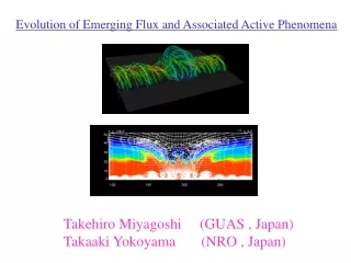
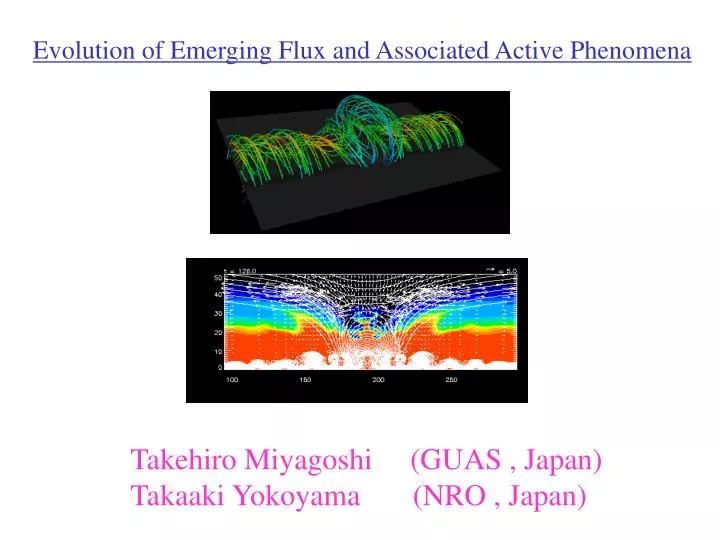
Evolution of Emerging Flux and Associated Active Phenomena. Takehiro Miyagoshi (GUAS , Japan) Takaaki Yokoyama (NRO , Japan). Studies of Coronal Magnetic Structure Formed by Isolated Twisted Emerging Flux by MHD Numerical Simulations. Upper Convection Zone --- Corona.

E N D
Evolution of Emerging Flux and Associated Active Phenomena Takehiro Miyagoshi (GUAS , Japan) Takaaki Yokoyama (NRO , Japan)
Studies of Coronal Magnetic Structure Formed by Isolated Twisted Emerging Flux by MHD Numerical Simulations • Upper Convection Zone --- Corona Initially, • Gold-Hoyle type twisted flux is • embedded in upper convection • zone • Magnetohydrostatic State • Small Perturbation is imposed • in the center region of the tube • at t=0 to excite instability Initial Condition of Numerical Simulations
Gold-Hoyle Type Force-Free Field These are forms of GH type force free field. The parameter ‘q’ is the strength of the twists. Today, we introduce results of two parameter cases, which are weak twist case (q=0.2) and strong twist case (q=1.0).
Case of q=0.2 Simulation Result: Time development of magnetic lines of force. Gray plane shows the surface of the Sun. Blue tubes show upper flux of the tube, and yellow show bottom flux of the tube.
Top View of Magnetic Lines of Force y x This is the last statement of the previous movie. (Right) top view of the magnetic lines of force. The characteristic helical structure fields are shown (yellow tubes).
Convection Motion near both Footpoints z x y The reason why the helical structure is formed is as follows: These are velocity fields and density map on the orthogonal slicer. (Emerging flux exists at the center.) As flux emerges, convection motion occurs near both footpoints of the tube. As flux tube emerges, plasma is lifted up by the emerging motion and fall down by gravity, and convection motion occurs by this process near both footpoints.
Schematic Picture and Comparison with Two-Dimensional Case (b) (a) (c) (a) Schematic picture of the process of forming helical structure. Convection motion pushes flux toward the center, and magnetic reconnection occurs. Then helical structure is produced at the center. (b) Expanded image near the helical structure. This process occur mainly in high beta region because magnetic flux is easily affected by convection motion at there. (c) Comparison with two dimensional case. (Parameters are almost same as 3D case). White lines show magnetic fields and white arrows show velocity fields. Magnetic flux is not tube but sheet in this case. But physical key process is same as 3D case. Magnetic island is formed in this case. In 3D case, This corresponds to magnetic helical structure because tube is s slightly twisted and has y components.
Case of q=1.0 This is the simulation result of strong twist (q=1.0) case. Blue tubes show center flux of the tube, and yellow show bottom flux in the emerging region.
Time Development of Magnetic Lines of Force (b) (a) (c) (a) Initial condition, (b) The last statement of the previous movie, (c) The top view of magnetic lines of force. The center flux (blue tube) forms S-shaped structure and bottom flux (yellow) is nearly normal to the blue flux.
Velocity Fields on the xy plane y Initial Perturbed Region x (Time development of yellow fields) This is velocity fields (blue arrows) and magnetic fields from top view (xy plane). The pink arrow shows initial perturbed region. In this case, flux is strongly twisted in the perturbed region. Convection motion also occur near both footpoints in this case and pushes flux toward the center. In this case, Yellow flux moves as shown in this figure as time development, and antiparallel component does not touch in this case by initial strong twist geometry.
Interaction between Emerging Flux & Coronal Field Coronal X-ray Jets : Yohkoh SXT Observation 1. 2. 3. Chromosphere Evaporation Flow Reconnection Outflow Reconnection Region Heat Conduction (Shibata et al. 1994) Next interesting problem is interaction between emerging flux and coronal fields. Emerging flux causes many active phenomena in the corona. We investigate interaction between emerging flux and overlying coronal fields as coronal jets based on this model. First, emerging flux reaches the height of coronal fields. Then magnetic reconnection occur between emerging flux and coronal fields, and magnetic energy is converted into thermal energy. This thermal energy is transported by heat conduction and evaporation jets are produced.
Numerical Simulation Results (Density and Magnetic Fields) Simulation result: time development of magnetic fields, velocity fields, and density. Emerging flux loop from the convection zone expands in the corona and reaches to the coronal field. Then reconnection starts and the released thermal energy conducts along the loops. Next, dense evaporation jet flow occurs along reconnected flux. We derived the parameter dependence of the jet mass by balance between conduction flux from loop top and enthalpy flux of the jet. We found that it nearly matches Yohkoh observation results (by Shimojo et al. 2000).
Existence of Two Type Jets Reconnection Jets (High Speed, Low Density) Evaporation Jets (Low speed, High Density) Simulation results show that two type jets exist around emerging flux region simultaneously. There are evaporation jets and reconnection jets. Evaporation jets are produced along reconnected flux. Reconnection jets are produced by reconnection outflow. Evaporation jets are low speed and high density, while reconnection jets are high speed and low density. Jets observed by Yohkoh is thought to be evaporation jets. We expect that these two type jets and their relation are cleared by collaboration observation by EIS and XRT.
Another problem : Interaction between twisted tube and coronal field We deal with interaction between emerging flux sheet and overlying coronal magnetic fields. (Shibata,K., & Uchida,Y. 1986) (Shimojo,M., 2002) Another interesting problem is interaction between flux tube and coronal open field. If flux tube is strongly twisted, magnetic pressure gradient works well after reconnection occurred, and torsional Alfven wave propagates along coronal open field. This would be observed helical motion jet. Examples of these helical jets exists (TRACE or Hα observation).
Summary Emerging Flux --- Our numerical simulations show that if flux tube is not strongly twisted itself, helical structure appears in the upper atmosphere. To see evolution of upper, center, and lower part of the emerging flux tube, to clear relation between magnetic structure of photosphere and upper atmosphere is very important. These can be cleared by collaboration observation of SOT and EIS. Reconnection Jets and Evaporation Jets --- The structures and relations between these two type jets around emerging flux region can be cleared by collaboration observation of EIS and XRT.
Initial Condition Corona Gravity Transition Region Choromosphere Photosphere Upper Convection Zone initial perturbed region magnetic fluxes MHD + Anisotropic Heat Conduction +Anomalous Resistivity
(With Heat Conduction Effect) (Without Heat Conduction Effect)
Mass of the Evaporation Jets: Comparison with Observations (From Observations) Density of the Jets Density of Flares at Footpoint (From our Numerical Simulation) (Shimojo et al. 2000)
シミュレーション結果から得られた依存性は、何をシミュレーション結果から得られた依存性は、何を 表しているか? (ジェットフローのエンタルピーフラッ クスと熱伝導フラックスのつり合い)
フレアの温度の見積もり (加熱と熱伝導のつり合い) リコネクショ ンによる加熱 フラックス