Download
1 / 25
270 likes | 493 Views
Image processing . Lecture 3. Important concepts (From the previous lectures) Image size

E N D
Image processing Lecture 3
Important concepts (From the previous lectures) • Image size • Image size of a bitmapped image can be described by the horizontal (H) and vertical (V) pixel count. The total number of pixels in an image is found by multiplying the horizontal and vertical pixel counts: • Total pixel count=HxV • Color Depth • Each pixel of the image contains unique color information. The a mount of color information is the color depth therefore, it is described in the unit of bits. Where • b= number of bits. • 2b =number of possible display colors.
In a 1 bit image (b=1) each pixel has either a 0 or 1 to code color so only two colors (21=2) black or white. • An 8-bit image uses 8 places of binary code to code for the colors. That allows a palette of 28=256 colors or 256 shades of gray. • A 24-bit color image works with a palette of over 16.7 million colors (i.e., 224=16700000). • Raw File Size • The image size combined with color depth gives the raw file size, the raw file size can be though of as a volume. We multiply the horizontal (H) pixel count by the vertical (V ) count by the color depth (D ) to get the raw file size: • Raw file size=HxVxD • Because all three of these variables are multiplied, • an increase in any of three adds to the file size.
Image Analysis Image analysis involves manipulating the image data to determine exactly the information necessary to help solve a computer imaging problem. This analysis is typically part of a larger process, is iterative in nature and allows us to answer application specific equations: Do we need color information? Do we need to transform the image data into the frequency domain? Do we need to segment the image to find object information? What are the important features of the image? Image analysis is primarily data reduction process. As we have seen, images contain enormous amount of data, typically on the order hundreds of kilobytes or even megabytes. Often much of this information is not necessary to solve a specific computer imaging problem, so primary part of the image analysis task is to determine exactly what information is necessary. Image analysis is used both computer vision and image processing.
For computer vision, the end product is typically the extraction of high-level information for computer analysis or manipulation. This high-level information may include shape parameter to control a robotics manipulator or color and texture features to help in diagnosis of a skin tumor. In image processing application, image analysis methods may be used to help determine the type of processing required and the specific parameters needed for that processing. For example, determine the degradation function for an image restoration procedure, developing an enhancement algorithm and determining exactly what information is visually important for image compression methods.
System Model The image analysis process can be broken down into three primary stages: Preprocessing. Data Reduction. Features Analysis. 1. Preprocessing Is used to remove noise and eliminate irrelevant, visually unnecessary information. Noise is unwanted information that can result from the image acquisition process, other preprocessing steps might include: • Gray –level or spatial quantization (reducing the number of bits per pixel or the image size). • Finding regions of interest for further processing.
2. Data Reduction: Involves either reducing the data in the spatial domain or transforming it into another domain called the frequency domain, and then extraction features for the analysis process. 3. Features Analysis: The features extracted by the data reduction process are examine and evaluated for their use in the application. After preprocessing we can perform segmentation on the image in the spatial domain or convert it into the frequency domain via a mathematical transform. After these processes we may choose to filter the image. This filtering process further reduces the data and allows us to extract the feature that we may require for analysis.
Preprocessing • The preprocessing algorithms, Techniques had operators that used to perform initial processing that makes the primary data reduction and analysis task easier. • They include operations related to • extracting regions of interest. • -performing basic algebraic operations on images. • enhancing specific image features. • reducing data in both resolution and brightness. • Preprocessing is a stage where the requirements are typically obvious and simple, such as the elimination of image information that is not required for the application.
Regions Of Interest(ROI) Often, for image analysis , we want to investigate more closely a specific area within the image, called Regions Of Interest(ROI) . to do this we need operations that modify the spatial coordinates for the image of the image, and these are categories as image geometry operations. the image geometry discussed here is crop, zoom, shrink, translate and rotate. the cutting it away from the rest of the image. After we have cropped the subimage from the original image,wecan zoom in on it by enlarging it.
Zoom The image crop process is the process of selecting a small portion of the image, a sub image and cutting it away from the rest of the image. After we have cropped a sub image from the original image we can zoom in on it by enlarge it. The zoom process can be done in numerous ways: 1. Zero-Order Hold. 2. First _Order Hold. 3.Convolution. 1. Zero-Order hold: is performed by repeating previous pixel values, thus creating a blocky effect as in the following figure:
REPEAT Rows REPEAT Colms
2. First _Order Hold: is performed by finding linear interpolation between a adjacent pixels, i.e., finding the average value between two pixels and use that as the pixel value between those two, we can do this for the rows first as follows: The first two pixels in the first row are averaged (8+4)/2=6, and this number is inserted between those two pixels. This is done for every pixel pair in each row.
Next, take result and expanded the columns in the same way as follows:
3- Convolution: this process requires a mathematical process to enlarge an image. This method required two steps: Extend the image by adding rows and columns of zeros between the existing rows and columns. Perform the convolution.
Next, we use convolution mask, which is slide a cross the extended image, and perform simple arithmetic operation at each pixel location The convolution process requires us to overlay the mask on the image, multiply the coincident (متقابلة)values and sum all these results. This is equivalent to finding the vector inner product of the mask with underlying sub image. The vector inner product is found by overlaying mask on sub image. Multiplying coincident terms, and summing the resulting products.
For example, if we put the mask over the upper-left corner of the image, we obtain (from right to left, and top to bottom): 1/4(0) +1/2(0) +1/4(0) +1/2(0) +1(3) +1/2(0) + 1/4(0) +1/2(0) +1/4(0) =3 Notethat the existing image values do not change. The next step is to slide the mask over by on pixel and repeat the process, as follows: 1/4(0) +1/2(0) +1/4(0) +1/2(3) +1(0) +1/2(5) + 1/4(0) +1/2(0) +1/4(0) =4 Notethis is the average of the two existing neighbors. -This process continues until we get to the end of the row, each time placing the result of the operation in the location corresponding to center of the mask. -When the end of the row is reached, the mask is moved down one row, -and the process is repeated row by row. This procedure has been performed on the entire image, the process of sliding, multiplying and summing is called convolution.
Note that the output image must be put in a separate image array called a buffer, so that the existing values are not overwritten during the convolution process. a. Overlay the convolution mask in the upper-left corner of the image. Multiply coincident terms, sum, and put the result into the image buffer at the location that corresponds to the masks current center, which is (r,c)=(1,1).
b. Move the mask one pixel to the right , multiply coincident terms sum , and place the new results into the buffer at the location that corresponds to the new center location of the convolution mask which is now at (r,c)=(1,2), continue to the end of the row. c. Move the mask down on row and repeat the process until the mask is convolved with the entire image. Note that we lose the outer row(s) and columns(s).
Why we use this convolution method when it require, so many more calculation than the basic averaging of the neighbors method? Note, only first-order hold be performed via convolution, but zero-order hold can also achieved by extending the image with zeros and using the following convolution mask. Note that for this mask we will need to put the result in the pixel location corresponding to the lower-right corner because there is no center pixel. These methods will only allows us to enlarge an image by a factor of (2N-1), but what if we want to enlarge an image by something other than a factor of (2N-1)?
3.Convolution Zero padded 1 The mask 2 0*1/4+ 0*1/2+ 0*1/4+ 0*1/2+ 3*1+ 0*1/2+ 0*1/4+ 0*1/2+ 0*1/4 3 0*1/4+ 0*1/2+ 0*1/4+ 3*1/2+ 3*1+ 5*1/2+ 0*1/4+ 0*1/2+ 0*1/4 4 0*1/4+ 0*1/2+ 0*1/4+ 0*1/2+ 5*1+ 0*1/2+ 0*1/4+ 0*1/2+ 0*1/4 5
0*1/4+ 3*1/2+ 4*1/4+ 0*1/2+ 0*1+ 0*1/2+ 0*1/4+ 2*1/2+ 0*1/4 ???? 3*1/4+ 4*1/2+ 5*1/4+ 0*1/2+ 0*1+ 0*1/2+ 2*1/4+ 0*1/2+ 7*1/4 ????? 4*1/4+ 5*1/2+ 0*1/4+ 0*1/2+ 0*1+ 0*1/2+ 0*1/4+ 7*1/2+ 0*1/4 ??
0*1/4+ 0*1/2+ 0*1/4+ 0*1/2+ 2*1+ 4.5*1/2+ 0*1/4+ 0*1/2+ 0*1/4 2 0*1/4+ 0*1/2+ 0*1/4+ 2*1/2+ 4.5*1+ 7*1/2+ 0*1/4+ 0*1/2+ 0*1/4 9/2 0*1/4+ 0*1/2+ 0*1/4+ 4.5*1/2+ 7*1+ 0*1/2+ 0*1/4+ 0*1/2+ 0*1/4 7
Zoom Using K-factor To do this we need to apply a more general method. We take two adjacent values and linearly interpolate more than one value between them. This is done by define an enlargement number k and then following this process: 1. Subtract the values. 2. Divide the result by k. 3. Add the result to the smaller value, and keep adding the result from the second step in a running total until all (k-1) intermediate pixel locations are filled.
Example: 1. Find the difference between the two values, 140-125 =15. we want to enlarge an image to three times its original size, and we have two adjacent pixel values 125 and 140. 2. The desired enlargement is k=3, so we get 15/3=5. 3. next determine how many intermediate pixel values .we need : K-1=3-1=2. The two pixel values between the 125 and 140 are 125+5=130 and 125+2*5 = 135. • We do this for every pair of adjacent pixels .first along the rows and then along the columns. This will allows us to enlarge the image by any factor of K (N-1) +1 where K is an integer and N×N is the image size.