Download
1 / 48
480 likes | 583 Views
FCH 532 Lecture 7. Chapter 5: DNA sequencing Chapter 7 2 new HW assignments Test next Friday. Genome sequencing. In order to sequence entire genomes, segments need to be assembled into contigs (contiguous blocks) to establish the correct order of the sequence.

E N D
FCH 532 Lecture 7 Chapter 5: DNA sequencing Chapter 7 2 new HW assignments Test next Friday
Genome sequencing • In order to sequence entire genomes, segments need to be assembled into contigs (contiguous blocks) to establish the correct order of the sequence. • Chromosome walking may be one way to do so, but is prohibitively expensive. • Two methods have been used recently: • 1. Conventional genome sequencing-low resolution maps made by identifying “landmarks” in ~250 kb inserts in YACs. • Landmarks are 200-300 bp segments, aka sequence tagged sites(STSs)-2 clones with the same STS overlap. • STS-containing inserts are sheared randomly into ~40kB segments and cloned into cosmid vectors-used to create high resolution maps. • The cosmid inserts are fragmented to smaller sizes and sequenced. • Cosmid inserts are assembled by using the STS sequence overlaps and cosmid walking. • Cannot be used effectively with sequences containing high amounts of repetitive sequence. (Use expressed sequence tags (ESTs)).
Genome sequencing • 2. Shotgun strategy- • genome library is randomly fragmented • large amount of cloned fragments are sequenced. • Genome is assembled by identifying overlaps between pairs of fragments. • The probability that a base is not sequenced is e-c, • c is the redundancy of coverage, c = LN/G, • where L is the average length of the cloned inserts in base pairs, • N is the number of inserts sequenced, • and G is the length of the genome in base pairs. • The aggregate length of the gaps between contigs is G e-cand the average gap size is G/N. • Bacterial genomes-shotgun strategy is straightforward. Gaps are filled in by synthesizing PCR primers and finishing a genome. • Eukaryotic genomes-larger size so it must be carried out in stages using BACs and then identifying ~500 bp sequences from each to yield sequence tagged connnectors (STCs or BAC ends) • This allows assembly via the overlapping of STCs.
Human genome • 2.2 billion nucleotide sequence ~90% complete because of highly repetitive sequence. • About half of the human genome consists of various repeating sequences. • Only ~28% of the genome is transcribed to RNA • Only 1.1% to 1.4% of the genome (~5% of the transcribed RNA) encodes protein. • Only ~30,000 protein encoding genes (open reading frames or ORFs) identified. Predicted 50,000 - 140,000 ORFs. • Only a small fraction of human protein families are unique to vertebrates; most occur in other life forms. • Two randomly selected human genomes differ, on average, by only 1 nucleotide per 1250; that is, any 2 people are likely to be >99.9% identical.
Human genome • 2.2 billion nucleotide sequence ~90% complete because of highly repetitive sequence. • About half of the human genome consists of various repeating sequences. • Only ~28% of the genome is transcribed to RNA • Only 1.1% to 1.4% of the genome (~5% of the transcribed RNA) encodes protein. • Only ~30,000 protein encoding genes (open reading frames or ORFs) identified. Predicted 50,000 - 140,000 ORFs. • Only a small fraction of human protein families are unique to vertebrates; most occur in other life forms. • Two randomly selected human genomes differ, on average, by only 1 nucleotide per 1250; that is, any 2 people are likely to be >99.9% identical.
Chemical evolution • Evolutionary aspects of amino acid sequences. • Change stem from random mutational events that alter a protein’s primary structure. • Mutational change must offer a selective advantage or at least, not decrease fitness. • Most mutations are deleterious and often lethal so they are not reproduced. • Sometimes mutations occur that increase fitness of the host in its natural environment. • Example: Sickle-cell anemia.
Figure 7-18a Scanning electron microscope of human erythrocytes. (a) Normal human erythrocytes revealing their biconcave disklike shape. Page 183
Figure 7-18b Scanning electron microscope of human erythrocytes. (b) Sickled erythrocytes from an individual with sickle-cell anemia. Page 183
Figure 7-20 A map indicating the regions of the world where malaria caused by P. falciparum was prevalent before 1930. Page 184
Chemical evolution • Pauling and co-workers showed that normal human hemoglobin (HbA) is more electronegative than sickle-cell hemoglobin (HbS). • Sickle-cell anemia is inherited according to the laws of Mendelian genetics. • Homozygous for HbS is almost all HbS, phenotype=sickle cell anemia. • Heterozygous for HbS is ~40% HBs, phenotype=sickle cell trait. • Homozygous for HbA, normal human hemoglobin.
Mutations ina-orb-globin genes can cause disease state • Sickle cell anemia – E6 to V6 • Causes V6 to bind to hydrophobic pocket in deoxy-Hb • Polymerizes to form long filaments • Cause sickling of cells • Sickle cell trait offers advantage against malaria • Cells sickle under low oxygen conditions and if infected with Plasmodium falciparum. • Causes the preferential removal of infected erythrocytes from circulation.
Variations in homologous proteins • Similar proteins from related species likely derived from the same ancestor. • A protein that is well adapted to its function will continue to evolve. • Neutral drift-mutational changes in a protein that don’t affect its function over time. • Homologous proteins-evolutionarily related proteins. • Comparison of the primary structures of homologous structures can be used to identify which residues are essential to its function, lesser significance, and little function. • Invariant residue-the same side chain at a particular position in the amino acid sequence of related proteins. • If an invariant residue is observed between related proteins, it is likely necessary to some essential function of the protein. • Other amino acids may have less stringent side chain requirements-where amino acids may be conservatively substituted-(be substituted with an amino acid with similar properties). • If many amino acids tolerated at a specific position - hypervariable.
Cytochrome c • Cytochrome c is nearly universal eukaryotic protein necessary for electron transport. • Vertebrates 103-104 residues; up to 8 more aas in other phyla. • Similarities are observed in an alignment. • 38 of 105 residues are invariant and the others are conservatively substituted. • 8 positions are hypervariable. • His 18 and Met 80 form bonds with the redox Fe of the heme group.
Table 7-4a Amino Acid Sequences of Cytochromes c from 38 species. Page 184
Cytochrome c • Evolutionary differences between two homologous proteins are determined by counting the amino acid differences between them. • Order of differences parallels taxonomy and can be put into a table. • This data can be used to construct a phylogenetic tree-a tree that indicates ancestral relationships among organisms and their proteins.
Figure 7-21 Phylogenic tree of cytochrome c. • Each branch point indicates a possible common ancestor to everything above it. • Relative evolutionary distances between neighboring branch points are expressed as the number of amino acid differences per 100 residues of the protein (percentage of accepted point mutations or PAM units). Page 187
Evolutionary rates • Evolutionary distances between various species can be plotted against the time when species diverged. • Each protein has a characteristic rate of change-unit evolutionary period-the time required for the amino acid sequence of the protein to change by 1% after two species have diverged. • Acceptance rate of mutations depends on the extent to which amino acid affects function. • Amino acid substitutions in a protein mostly result from single base changes in the gene specifying the protein (point mutations). • Point mutations in DNA accumulate at a constant rate with time-resulting from random chemical change rather than errors from the replication process.
Figure 7-22 Rates of evolution of four unrelated proteins. Tolerant Page 188 Intolerant of changes
Evolutionary rates • Amino acid substitutions in a protein mostly result from single base changes in the gene specifying the protein (point mutations). • Point mutations in DNA accumulate at a constant rate with time-resulting from random chemical change rather than errors from the replication process. • Know this based on generation times of different organisms.
Evolutionary rates • Protein evolution is not the basis for organismal evolution. • Rapid divergence is likely due to mutational changes in DNA that control gene expression. • Some proteins have extensive sequence similarity in the same organism resulting from a gene duplication. • Gene duplication is an efficient mode of evolution because the new gene can evolve a new functionality while the original directs synthesis of the ancestral protein. • Globins-an example-see Ch. 7. • Paralog-homologous proteins in the same organism • Orthologs-homologous proteins/genes in different organisms that arose through species divergence.
Bioinformatics • Biotechnology meets computer science. • Sequence databases
Sequence alignment • Sequence similarity of two polypeptides or two DNAs can be quantified by determining the number of aligned residues that are identical. • Human and dog cytochromes c differ in 11 or 104 residues [(104-11)/104] X 100=89% identical. • Human and yeast are [(104-45)/104] X 100 = 57% identical. • When determining percent identity, the length of the shorter peptide/DNA is by convention, used in the denominator. • Must also decide which amino acid residues are considered similar (e.g. Asp and Glu).
Homology of distantly related proteins • Hypothetical example: Assume that we have a 100 residue protein in which all point mutations have equal probability of being accepted and happen at a constant rate. • At an evolutionary distance of 1 PAM unit, the original and evolved proteins are 99% identical. • At an evolutionary distance of 2 PAM units, they are (0.99)2 X 100 = 98% identical • At 50 PAM units, they are (0.99)50 X 100 = 60.5% identical. • This is due to the stochastic (random) process of mutation. Every residue has an equal chance of mutating. • These can be plotted as percent identity vs. evolutionary distance.
Figure 7-25a Rate of sequence change in evolving proteins. (a) Protein evolving at random and that initially consists of 5% each of the 20 “standard” amino acid residues. Approaches but never = 0! Page 193
Homology of distantly related proteins • Real proteins are more complex. • Certain amino acids are more likely to be accepted than others. • Distribution of amino acids in proteins is not uniform (9.5% are Leu on average and only 1.2% are Trp). • Can also be affected by shifts in the sequence resulting from insertion or deletion of one or more residues within a chain. • Example is different lengths of cytochrome c peptides. • If the amino acid sequence is allowed to shift, the best alignment will increase.
SQMCILFKAQMNYGH MFYACRLPMGAHYWL Unlimited gapping SQMCILFKAQMNYGH --M---F-----YACRLPMGAHYWL Homology of distantly related proteins • Unlimited gapping because of insertions and deletions (indels) cannot be allowed because we won’t get the proper alignment. • At the same time we need to allow for gapping (cyt c). • There must be a penalty for gaps. • Unrelated proteins will exhibit sequence identities (15-25%) which will be the same as distantly related proteins. • Requires more sophisticated algorithms to describe
Figure 7-25b Rate of sequence change in evolving proteins. (b) A protein of average amino acid composition evolving as is observed in nature. Area in which unrelated and distantly related proteins have sequence identity (15%-25%) Page 193
Sequence alignments • Pairwise sequence alignments can be done by using a dot matrix. • One sequence is plotted horizontally and the other vertically. Whenever there is an identical residue you place a dot on the chart. • Dot plot of a peptide against itself results in a square matrix with a row of dots along the diagonal and scattered dots for chance identities. • If the peptides are conserved, there are only a few absences along the diagonal. • Distantly related peptides will have a number of gaps along the diagonal.
Sequence alignments • An alignment score (AS)is used to determine if there is any relationship. • 10 for every identity except Cys which scores 20 • Subtract 25 for every gap. • The normalized alignment score (NAS) by dividing the AS by the number of residues of the shortest of the two polypeptides in the alignment and multiplying by 100. • Example Human hemoglobin and myoglobin.
Figure 7-27 The optical alignments of human myoglobin (Mb, 153 residues) and the human hemoglobin a chain (Hba, 141 residues). Hemoglobin is 141 and myoglobin is 153 AS = number of identities X 10 + 20 for Cys -number of gaps = 37 identities X 10 + 20 (Cys) - (1gap X 25)= 365 NAS = AS/number of residues for shortest polypeptide =365/141 = 259 Page 195
Figure 7-28 A guide to the significance of normalized alignment scores (NAS) in the comparison of peptide sequences. Page 195
Alignments are weighted according to the likelihood of substitution • Realistic way of assigning the probability of occurrence (weight) for a substitution is to look at the physical similarity of amino acids. • Dayhoff measured a number of residue exchanges for closely related proteins and determined their relative frequency of the 20 X 19/2 = 190 different possible residue changes. • This number is divided by 2 to account for the fact that A B and B A are equally likely. • These data can be used to create a square matrix (20 X 20) • The elements (20 properties per side) Mij, indicate the probability that, in a related sequence, amino acid i will replace amino acid j after an evolutionary interval (usually one PAM unit). • PAM-1 matrix.
PAM matrix • Mutation probability can be determined for other evolutionary distances. • PAM-N matrix is made bt multiplying the matrix by itself N times ([M]N). • Relatedness odds matrix - Rij = Mij/fi • fi = probability that the amino acid i will occur in the second sequence by chance. • Rij = probability that amino acid i will replace amino acid j or vice versa every time i or j is encountered in the sequence. • When two polypeptides are compared with each other, the Rij values for each position are multiplied to give the relatedness odds. • For example A-B-C-D-E-F and P-Q-R-S-T-U, relatedness odds = RAP X RBQ X RCR X RDS X RET X RFU • Log odds substitution matrix - is made by taking the log of the relatedness odds. • Log odds need to be maximized to get the best alignment.
Table 7-7 The PAM-250 Log Odds Substitution Matrix. All elements multiplied by 10. Each diagonal element indicates the mutability of the corresponding amino acid. Neutral score = 0. Page 196
Sequence alignment • Make a matrix with the log odds values associated with the amino acids at the appropriate positions. • Example use a PAM-250 log odds matrix with a 10 peptide horizontal and 11 peptide vertical. • The alignment of these two peptides must have at least one gap assuming a significant alignment can be found. • This is called a comparison matrix
Figure 7-29a Use of the Needleman-Wunsch alignment algorithm [alignment of 10-residue peptide (horizontal) with 11-residue peptide (vertical)]. (a) Comparison matrix. Page 197
Needleman-Wunsch algorithm • Needleman and Wunsch constructed an algorithm to find the best alignment between 2 polypeptides. • Start at the lower right corner of the matrix (C-termini) at position M and N (these correspond to the 10th and 11th amino acid residues) and add the value to the position M-1, N-1 in the matrix. • Add to each element of the matrix the largest number from the row or column to the lower right of each element proceeding right to left, bottom to top.
Figure 7-29b Use of the Needleman-Wunsch alignment algorithm [alignment of 10-residue peptide (horizontal) with 11-residue peptide (vertical)]. (b) Transforming the matrix. Page 197