Download
1 / 59
590 likes | 679 Views
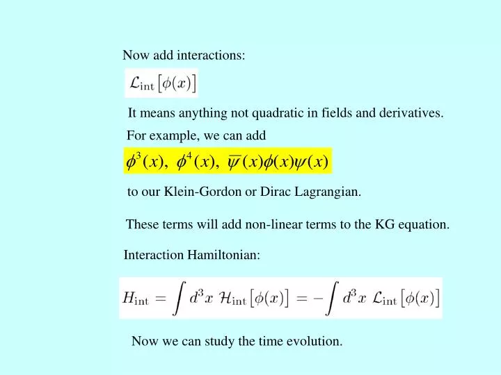
Now add interactions:. It means anything not quadratic in fields and derivatives. For example, we can add. to our Klein-Gordon or Dirac Lagrangian. These terms will add non-linear terms to the KG equation. Interaction Hamiltonian:. Now we can study the time evolution. Schrodinger Picture.

E N D
Now add interactions: It means anything not quadratic in fields and derivatives. For example, we can add to our Klein-Gordon or Dirac Lagrangian. These terms will add non-linear terms to the KG equation. Interaction Hamiltonian: Now we can study the time evolution.
Schrodinger Picture States evolve with time, but not the operators. It is the default choice in wave mechanics. 狀態 波函數 測量 算子 Evolution Operator:
Only the expectation values are observable. For the same evolving expectation value, we can instead ask operators to evolve. Heisenberg Picture Now the states do not evolve. We move the time evolution to the operators: Heisenberg Equation The rate of change of operators equals their commutators with H.
Combine the two eq. KG Equation
Interaction picture We can move just the free H0 to operators. States and Operators both evolve with time in interaction picture: S
Evolution of Operators Operators evolve just like operators in the Heisenberg picture but with the full Hamiltonian replaced by the free Hamiltonian For field operators in the interaction picture: Field operators are free, as if there is no interaction! The Fourier expansion of a free field is still valid.
Evolution of States S States evolve like in the Schrodinger picture but with Hamiltonian replaced by HI(t). HI(t) is just the interaction Hamiltonian Hint in interaction picture! That means, the field operators in HI(t) are free.
Interaction Picture Operators evolve just like in the Heisenberg picture but with the full Hamiltonian replaced by the free Hamiltonian States evolve like in the Schrodinger picture but with the full Hamiltonian replaced by the interaction Hamiltonian.
U operator, the evolution operator of states in the interaction picture Define time evolution operator U All the problems can be answered if we are able to calculate this operator. It determines the evolution of states.
is the state in the future t which evolved from a state ψ in t0 is the state in long future which evolved from a state ψ from long past. The amplitude for this state to appear as a state ϕ is their inner product: The transition amplitude for the decay of A: can be computed: The transition amplitude for the scattering of A: can be computed:
Perturbation expansion Solve it by a perturbation expansion in small parameters in HI. To leading order:
Define S matrix: It is Lorentz invariant if the interaction Lagrangian is invariant.
Vertex In ABC model, every particle corresponds to a field: Add an interaction term in the Lagrangian: The transition amplitude for the decay of A: can be computed: To leading order:
The remaining numerical factor is: B C Momentum Conservation ig A
For a toy ABC model Three scalar particle with masses mA, mB ,mC 1 External Lines Internal Lines Lines for each kind of particle with appropriate masses. C -ig Vertex A B The configuration of the vertex determine the interaction of the model.
A B C interaction Lagrangian vertex Every field operator in the interaction corresponds to one leg in the vertex. Every field is a linear combination of a and a+ Every leg of a vertex can either annihilate or create a particle! This diagram is actually the combination of 8 diagrams!
A B C Interaction Lagrangian vertex The Interaction Lagrangian is integrated over the whole spacetime. Interaction could happen anywhere anytime. The amplitudes at various spacetime need to be added up. The integration yields a momentum conservation. In momentum space, the factor for a vertex is simply a constant.
Interaction Lagrangian Vertex Every field operator in the interaction corresponds to one leg in the vertex. Every leg of a vertex can either annihilate or create a particle!
Propagator Solve the evolution operator to the second order. HI is first order. The integration of two identical interaction Hamiltonian HI. The first HI is always later than the second HI
The integration of two identical interaction Hamiltonian HI. The first HI is always later than the second HI t’ and t’’ are just dummy notations and can be exchanged. t’’ We are integrating over the whole square but always keep the first H later in time than the second H. t’
t’’ This definition is Lorentz invariant! t’
This notation is so powerful, the whole series of operator U can be explicitly written: The whole series can be summed into an exponential:
Amplitude for scattering Fourier Transformation Propagator between x1 and x2 p2-p4 pour into C at x1 p1-p3 pour into C at x2
B(p3) B(p4) x1 C(p1-p3) x2 C A(p1) A(p2) A particle is created at x2 and later annihilated at x1. B(p4) B(p3) A(p1) A(p2)
B(p3) B(p4) x2 x1 C(p1-p3) x2 x1 C C A(p1) A(p2) A particle is created at x1 and later annihilated at x2. B(p4) B(p3) B(p4) B(p3) A(p1) A(p1) A(p2) A(p2)
B(p3) B(p4) x2 x1 C(p1-p3) x2 x1 C C A(p1) A(p2) B(p4) B(p3) B(p4) B(p3) A(p1) A(p1) A(p2) A(p2) This construction ensures causality of the process. It is actually the sum of two possible but exclusive processes. Again every Interaction is integrated over the whole spacetime. Interaction could happen anywhere anytime and amplitudes need superposition.
This propagator looks reasonable in coordinate space but difficult to calculate and the formula is cumbersome.
This doesn’t look explicitly Lorentz invariant. But by definition it should be! So an even more useful form is obtained by extending the integration to 4-momentum. And in the momentum space, it becomes extremely simple:
B(p3) B(p4) x2 x1 C(p1-p3) x2 x1 C C A(p1) A(p2) The Fourier Transform of the propagator is simple. B(p4) B(p3) B(p4) B(p3) A(p1) A(p1) A(p2) A(p2)
B(p3) B(p4) x2 x1 C(p1-p3) x2 x1 C C A(p1) A(p2) B(p4) B(p3) B(p4) B(p3) A(p1) A(p1) A(p2) A(p2)
For a toy ABC model Internal Lines Lines for each kind of particle with appropriate masses.
Every field either couple with another field to form a propagator or annihilate (create) external particles! Otherwise the amplitude will vanish when a operators hit vacuum!
For a toy ABC model Three scalar particle with masses mA, mB ,mC 1 External Lines Internal Lines Lines for each kind of particle with appropriate masses. C -ig Vertex A B The configuration of the vertex determine the interaction of the model.
Scalar Antiparticle Assuming that the field operator is a complex number field. The creation operator b+ in a complex KG field can create a different particle! The particle b+ create has the same mass but opposite charge. b+ create an antiparticle.
Complex KG field can either annihilate a particle or create an antiparticle! Its conjugate either annihilate an antiparticle or create a particle! The charge difference a field operator generates is always the same! So we can add an arrow of the charge flow to every leg that corresponds to a field operator in the vertex.
incoming particle or outgoing antiparticle incoming antiparticle or outgoing particle charge non-conserving interaction
incoming antiparticle or outgoing particle incoming particle or outgoing antiparticle charge conserving interaction
incoming antiparticle or outgoing particle incoming particle or outgoing antiparticle can either annihilate a particle or create an antiparticle! can either annihilate an antiparticle or create a particle!
U(1) Abelian Symmetry The Lagrangian is invariant under the field phase transformation invariant is not invariant U(1) symmetric interactions correspond to charge conserving vertices.
A If A,B,C become complex, they all carry charges! B C The interaction is invariant only if The vertex is charge conserving.
B(p3) B(p4) x1 C(p1-p3) x2 C A(p1) A(p2) Propagator: An antiparticle is created at x2 and later annihilated at x1. B(p4) B(p3) A(p1) A(p2)
B(p3) B(p4) x2 x1 C(p1-p3) x2 x1 C C A(p1) A(p2) A particle is created at x1 and later annihilated at x2. B(p4) B(p3) B(p4) B(p3) A(p1) A(p1) A(p2) A(p2)
B(p3) B(p4) x2 x1 C(p1-p3) x2 x1 C C A(p1) A(p2) B(p4) B(p3) B(p4) B(p3) A(p1) A(p1) A(p2) A(p2)