Download
1 / 27
270 likes | 444 Views
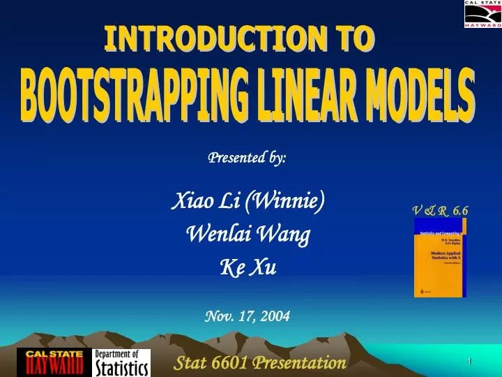
INTRODUCTION TO. BOOTSTRAPPING LINEAR MODELS. V & R 6.6. Stat 6601 Presentation. Presented by: Xiao Li (Winnie) Wenlai Wang Ke Xu Nov. 17, 2004. Bootstrapping Linear Models. 11/17/2004. Preview of the Presentation. Introduction to Bootstrap Data and Modeling

E N D
INTRODUCTION TO BOOTSTRAPPING LINEAR MODELS V & R 6.6 Stat 6601 Presentation Presented by: Xiao Li (Winnie) Wenlai Wang Ke Xu Nov. 17, 2004
Bootstrapping Linear Models 11/17/2004 Preview of the Presentation • Introduction to Bootstrap • Data and Modeling • Methods on Bootstrapping LM • Results • Issues and Discussion • Summary
Bootstrapping Linear Models 11/17/2004 What is Bootstrapping ? • Invented by Bradley Efron, and further developed by Efron and Tibshirani • A method for estimating the sampling distribution of an estimator by resampling with replacement from the original sample • A method to determine the trustworthiness of a statistic (generalization of the standard deviation)
Bootstrapping Linear Models 11/17/2004 Why uses Bootstrapping ? • Start with 2 questions: • What estimator should be used? • Having chosen an estimator, how accurate is it? • Linear Model with normal random errors having constant variance Least Square • Generalized non-normal errors and non-constant variance ???
Bootstrapping Linear Models 11/17/2004 The Mammals Data • A data frame with average brain and body weights for 62 species of land mammals. • “body” : Body weight in Kg • “brain” : Brain weight in g • “name”: Common name of species
Bootstrapping Linear Models 11/17/2004 Data and Model Linear Regression Model: where j = 1, …, n, and is considered random y = log(brain weight) x = log(body weight)
See Code Bootstrapping Linear Models 11/17/2004 Summary of Original Fit Residuals: Min 1Q Median 3Q Max -1.71550 -0.49228 -0.06162 0.43597 1.94829 Coefficients: Estimate Std. Error t value Pr(>|t|) (Intercept) 2.13479 0.09604 22.23 <2e-16 *** log(body) 0.75169 0.02846 26.41 <2e-16 *** Residual standard error: 0.6943 on 60 DF Multiple R-Squared: 0.9208 Adjusted R-squared: 0.9195 F-statistic: 697.4 on 1 and 60 DF p-value: < 2.2e-16
Bootstrapping Linear Models 11/17/2004 for Original Modeling Code library(MASS) library(boot) c <- par(mfrow=c(1,2)) data <- data(mammals) plot(mammals$body, mammals$brain, main='Original Data', xlab='body weight', ylab='brain weight', col=’brown’) # plot of data plot(log(mammals$body), log(mammals$brain), main='Log-Transformed Data', xlab='log body weight', ylab='log brain weight', col=’brown’) # plot of log-transformed data mammal <- data.frame(log(mammals$body), log(mammals$brain)) dimnames(mammal) <- list((1:62), c("body", "brain")) attach(mammal) log.fit <- lm(brain~body, data=mammal) summary(log.fit)
Bootstrapping Linear Models 11/17/2004 Two Methods • Case-based Resampling: randomly sample pairs (Xi, Yi) with replacement • No assumption about variance homogeneity • Design fixes the information content of a sample • Model-based Resampling: resample the residuals • Assume model is correct with homoscedastic errors • Resampling model has the same “design” as the data
Bootstrapping Linear Models 11/17/2004 Case-Based Resample Algorithm For r = 1, …, R, • sample randomly with replacement from {1, 2, …,n} • for j = 1, …, n, set , then • fit least squares regression to , …, giving estimates , , .
Bootstrapping Linear Models 11/17/2004 Model-Based Resample Algorithm For r = 1, …, n, • For j = 1, … , n, • Set • Randomly sample from , …, ; then • Set • Fit least squares regression to ,…, giving estimates , , .
Compare Bootstrapping Linear Models 11/17/2004 Case-Based Bootstrap Output: ORDINARY NONPARAMETRIC BOOTSTRAP Bootstrap Statistics : original bias std. error t1* 2.134789 -0.0022155790 0.08708311 t2* 0.751686 0.0001295280 0.02277497 BOOTSTRAP CONFIDENCE INTERVAL CALCULATIONS Intervals : Level Normal Percentile BCa 95% ( 1.966, 2.308 ) ( 1.963, 2.310 ) ( 1.974, 2.318 ) 95% ( 0.7069, 0.7962 ) ( 0.7082, 0.7954 ) ( 0.7080, 0.7953 ) Calculations and Intervals on Original Scale
Bootstrapping Linear Models 11/17/2004 Case-Based Bootstrap Bootstrap Distribution Plots for intercept andSlope
Bootstrapping Linear Models 11/17/2004 Case-Based Bootstrap Standardized Jackknife-after-Bootstrap Plots for intercept andSlope
Bootstrapping Linear Models 11/17/2004 for Case-Based Code # Case-Based Resampling fit.case <- function(data) coef(lm(log(data$brain)~log(data$body))) mam.case <- function(data, i) fit.case(data[i, ]) mam.case.boot <- boot(mammals, mam.case, R = 999) mam.case.boot boot.ci(mam.case.boot, type=c("norm", "perc", "bca")) boot.ci(mam.case.boot, index=2, type=c("norm", "perc", "bca")) plot(mam.case.boot) plot(mam.case.boot, index=2) jack.after.boot(mam.case.boot) jack.after.boot(mam.case.boot, index=2) RANDOM!
Compare Bootstrapping Linear Models 11/17/2004 Model-Based Bootstrap Output: ORDINARY NONPARAMETRIC BOOTSTRAP Bootstrap Statistics : original bias std. error t1* 2.134789 0.0049756072 0.09424796 t2* 0.751686 -0.0006573983 0.02719809 BOOTSTRAP CONFIDENCE INTERVAL CALCULATIONS Intervals : Level Normal Percentile Bca 95% ( 1.945, 2.315 ) ( 1.948, 2.322 ) ( 1.941, 2.316 ) 95% ( 0.6990, 0.8057 ) ( 0.6982, 0.8062 ) ( 0.6987, 0.8077 ) Calculations and Intervals on Original Scale
Bootstrapping Linear Models 11/17/2004 Model-Based Bootstrap Bootstrap Distribution Plots for intercept andSlope
Bootstrapping Linear Models 11/17/2004 Model-Based Bootstrap Standardized Jackknife-after-Bootstrap Plots for intercept andSlope
Bootstrapping Linear Models 11/17/2004 Code for Model-Based # Model-Based Resampling (Resample Residuals) fit.res <- lm(brain ~ body, data=mammal) mam.res.data <- data.frame(mammal, res=resid(fit.res), fitted=fitted(fit.res)) mam.res <- function(data, i){ d <- data d$brain <- d$fitted + d$res[i] coef(update(fit.res, data=d)) } fit.res.boot <- boot(mam.res.data, mam.res, R = 999) fit.res.boot boot.ci(fit.res.boot, type=c("norm", "perc", "bca")) boot.ci(fit.res.boot, index=2, type=c("norm", "perc", "bca")) plot(fit.res.boot) plot(fit.res.boot, index=2) boot.ci(fit.res.boot, type=c("norm", "perc", "bca")) jack.after.boot(fit.res.boot) jack.after.boot(fit.res.boot, index=2) FIXED!
Bootstrapping Linear Models 11/17/2004 Comparisons and Discussion
Bootstrapping Linear Models 11/17/2004 Case-Based Vs. Model-Based • Model-based resampling enforces the assumption that errors are randomly distributed by resampling the residuals from a common distribution • If the model is not specified correctly – i.e., unmodeled nonlinearity, non-constant error variance, or outliers – these attributes do not carry over to the bootstrap samples • The effects of outliers is clear in the case-based, but not with the model-based.
FAIL Bootstrapping Linear Models 11/17/2004 When Might Bootstrapping Fail? • Incomplete Data • Assume that missing data are not problematic • If multiple imputation is used beforehand • Dependent Data • Bootstrap imposes mutual dependence on the Yj, and thus their joint distribution is • Outliers and Influential Cases • Remove/Correct obvious outliers • Avoid the simulations to depend on particular observations
Bootstrapping Linear Models 11/17/2004 Review & More Resampling • Resampling techniques are powerful tools for: -- estimating SD from small samples -- when the statistics do not have easily determined SD • Bootstrapping involves: -- taking ‘new’ random samples with replacement from the original data -- calculate boostrap SD and statistical test from the average of the statistic from the bootstrap samples • More resampling techniques: -- Jackknife resampling -- Cross-validation
Bootstrapping Linear Models 11/17/2004 SUMMARY • Introduction to Bootstrap • Data and Modeling • Methods on Bootstrapping LM • Results and Comparisons • Issues and Discussion
Bootstrapping Linear Models 11/17/2004 Reference • Anderson, B. “Resampling and Regression” McMaster University. http://socserv.mcmaster.ca/anderson • Davision, A.C. and Hinkley D.V. (1997) Bootstrap methods and their application. pp.256-273. Cambridge University Press • Efron and Gong (February 1983), A Leisurely Look at the Bootstrap, the Jackknife, and Cross Validation, The American Statistician. • Holmes, S. “Introduction to the Bootstrap” Stanford University. http://wwwstat.stanford.edu/~susan/courses/s208/ • Venables and Ripley (2002), Modern Applied Statistics with S, 4th ed. pp. 163-165. Springer
Thank You Applause Please Bootstrapping Linear Models 11/17/2004
Bootstrapping Linear Models 11/17/2004 Extra Stuff… • Jackknife Resampling takes new samples of the data by omitting each case individually and recalculating the statistic each time • Resampling data by randomly taking a single observation out • # of jackknife samples used # of cases in the original sample • Works well for robust estimators of location, but not for SD • Cross-Validation randomly splits the sample into two groups comparing the model results from one sample to the results from the other. • 1st subset is used to estimate a statistical model (screening/training sample) • Then test our findings on the second subset. (confirmatory/test sample)