Download
1 / 50
500 likes | 645 Views
CMRoboBits: Creating an Intelligent AIBO Robot. Instructors: Prof. Manuela Veloso & Dr. Paul E. Rybski TAs: Sonia Chernova & Nidhi Kalra 15-491, Fall 2004 http://www.andrew.cmu.edu/course/15-491 Computer Science Department Carnegie Mellon. AIBO Vision. Goals of this lecture

E N D
CMRoboBits: Creating an Intelligent AIBO Robot Instructors: Prof. Manuela Veloso & Dr. Paul E. Rybski TAs: Sonia Chernova & Nidhi Kalra 15-491, Fall 2004 http://www.andrew.cmu.edu/course/15-491 Computer Science Department Carnegie Mellon
AIBO Vision • Goals of this lecture • Illustrate the underlying processing involved with the AIBO vision system • Describe the high-level object recognition system • Provide enough background so that you can consider adding your own object detectors into the AIBO vision system
What is Computer Vision? • The process of extracting information from an image • Identifying objects projected into the image and determining their position • The art of throwing out information that is not needed, while keeping information needed • A very challenging research area • Not a solved problem!
AIBO Vision • AIBO camera provides images formatted in theYUV color space • Each image is an array of 176 x 144 pixels
Color Spaces • Each pixel is a 3 dimensional value • Each dimension is called a channel • There are multiple different possible color representations • RGB – R=red, G=green, B=blue • YUV – Y=brightness, UV=color • HSV – H=hue, S=saturation, V=brightness
Color Spaces - YUV • The AIBO camera provides images in YUV (or YCrCb) color space • Y – Luminance (brightness) • U/Cb – Blueness (Blue vs. Green) • V/Cr – Redness (Red vs. Green) • Technically, YUV and YCrCb are slightly different, but this does not matter for our purposes • We will refer to the AIBO color space as YUV
Color Spaces – HSV www.wordiq.com/definition/HSV_color_space
Color Spaces - Discussion • RGB • Handled by most capture cards • Used by computer monitors • Not easily separable channels • YUV • Handled by most capture cards • Used by TVs and JPEG images • Easily workable color space • HSV • Rarely used in capture cards • Numerically unstable for grayscale pixels • Computationally expensive to calculate
Image Raw R=Y G=U B=V
YUV Histogram Note: the U and V axes are swapped from the histogram in the previous slides (blue is in lower left corner in this slide but blue is in upper right corner in previous slide)
Vision Overview • CMRoboBits vision is divided into two parts • Low level • Handles bottom-up processing of image • Provides summaries of image features • High level • Performs top-down processing of image • Uses object models to filter low-level vision data • Identifies objects • Returns properties for those objects
Low-Level Vision Overview • Low level vision is responsible for summarizing relevant-to-task image features • Color is the main feature that is relevant to identifying the objects needed for the task • Important to reduce the total image information • Color segmentation algorithm • Segment image into symbolic colors • Run length encode image • Find connected components • Join nearby components into regions
Color Segmentation • Goal: semantically label each pixel as belonging to a particular type of object • Map the domain of raw camera pixels into the range of symbolic colors C • C includes ball, carpet, 2 goal colors, 1 additional marker color, 2 robot colors, walls/lines and unknown • Reduces the amount of information per pixel roughly by 1.8M • Instead of a space of 2563 values, we only have 9 values!
Color Segmentation Analysis • Advantages • Quickly extract relevant information • Provide useful representation for higher-level processing • Differentiate between YUV pixels that have similar values • Disadvantages • Cannot segment YUV pixels that have identical values into different classes • Generate smoothly contoured regions from noisy images
Turning Pixels into Regions • A disjoint set of labeled pixels is still not enough to properly identify objects • Pixels must be grouped into spatially-adjacent regions • Regions are grown by considering local neighborhoods around pixels N N N N 8-connected neighborhood 4-connected neighborhood N P N N P N N N N N
First Step : Run Length Encoding • Segment each image row into groups of similar pixels called runs • Runs store a start and end point for each contiguous row of color Original image RLE image
Final Results • Runs are merged into multi-row regions • Image is now described as contiguous regions instead of just pixels
Data Extracted from Regions • Features extracted from regions • Centroid • Mean location • Bounding box • Max and min (x,y) values • Area • Number of pixels in box • Average color • Mean color of region pixels • Regions are stored by color class and sorted by largest area • These features let us write concise and fast object detectors
High-Level Vision Overview • Responsible for finding relevant-to-task objects in image • Uses features extracted by low-level vision • Takes models of known objects and attempts to identify objects in the list of low-level regions • Generates a confidence of a region being the object of interest • Useful for differentiating between multiple classes • Generates an estimate of the object’s position in egocentric coordinates
Object Detection Process • Produces a set of candidate objects that might be this object from lists of regions • Given ‘n’ orange blobs, is one of them the ball? • Compares each candidate object to a set of models that predict what the object would look like when seen by a camera • Models encapulate all assumptions • Also called filtering • Selects best match to report to behaviors • Position and quality of match are also reported
Filtering Overview • Each filtering model produces a number in [0.0, 1.0] representing the certainty of a match • Some filters can be binary and will return either 0.0 or 1.0 • Certainty levels are multiplied together to produce an overall match • Real-valued range allows for areas of uncertainty • Keeps one bad filter result from ruining the object • Multiple bad observations will still cause the object to be thrown out
Example: Ball Detection • In robot soccer, having a good estimate of the ball is extremely important • A lot of effort has gone into good filters for detecting the ball position • Many filters are used in CMRoboBits • Most of these filters were determined by trial and error and hand-coded • Many filters contain “magic” numbers that work well in practice but do not necessarily have a theoretically sound basis
Ball – Filtering Models • Minimum size • Makes sure the ball has a bounding box at least 3 pixels tall and wide and 7 pixels total area • Square bounding box • Makes sure the bounding box is roughly square • Uses an unnormalized Gaussian as the output • Output is as follows: C=0.2 if on edge of image 0.6 otherwise
What Does the Filter Look Like? Filter Plot: o C=0.2 Plot: d H=10 W=[0-20] Plot: o C=0.6
Ball – Filtering Models • Area ratio • Compares the area covered by the pixels to the area covered by the bounding box • Elevation • Binary filter which ensures the ball is on the ground (less than 5 degrees in elevation) Area of ellipse with major and minor axes computed by bounding box C=0.2 if on edge of image 0.6 otherwise
Ball Distance Calculation • The size of the ball is known • The kinematics of the robot are known • Given a simplified camera projection model, the distance to the ball can be calculated
Pinhole Camera Model Object Image plane Image of object Pinhole camera
Inverted Pinhole Camera Model Object Image plane Focal length Image of object Inverted pinhole camera
Calculating Distance d Object Image plane f Image of object o i Inverted pinhole camera
Calculation of Camera Position • Position of camera is calculated based on body position and head position w.r.t body • Body position is known from walk engine • Head position relative to body position is found from forward kinematics using joint positions • Camera position • camera_loc is defined as position of camera relative to egocentric origin • camera_dir, camera_up, and camera_down are unit vectors in egocentric space • Specify camera direction, up and right in the image
Ball Position Estimation • Two methods are used for estimating the position of the ball • The first calculates the camera angle from the ball model • The second uses the robot’s encoders to calculate the head angle • The first is more accurate but relies on the pixel size of the ball • This method is chosen if the ball is NOT on the edge of the image • Partial occlusions will make this estimate worse
Ball Position Estimation • Ball position estimation problem is overconstrained. • g is the unknown camera a d h r g
Ball – Position Estimation • This method works all of the time • Camera angle computed from kinematics • Used when ball is on edge of image camera a h r g
Ball – Position Estimation • This method is more accurate • Requires accurate pixel count • Used only when ball is near center of image camera d h r g
Calculating Projection Error • Models the expected relative error in projection between the 2 ball estimation positions • Filters out candidate region if the two methods do not agree d=angular difference in camera angle between two methods
Additional Color Filters • The pixels around the ball are analyzed • Red vs. area • Filters out candidate balls that are part of red robot uniform • Green filter • Ensures the ball is near the green floor • If the ball is farther than 1.5m away • Average “redness” value of the ball is calculated • If too red, then the ball is assumed to be the fringe of the red robot’s uniform
Summary • Computer vision • Color spaces • Low-level vision • Color segmentation • Colored region extraction • High-level vision • Object filters • Example: tracking the ball