Download
1 / 27
280 likes | 363 Views
Implementing Particle Systems. CS 468 Spring 2004 Andrew Butts. What’s going on?. Just integrate the particle equations of motion. P’ = V V’ = A = F/m All the fun is in computing F… And in rendering!. Simulation Loop . PA 4 Requires this loop: Initialize/Emit particles

E N D
ImplementingParticle Systems CS 468 Spring 2004 Andrew Butts
What’s going on? • Just integrate the particle equations of motion. • P’ = V • V’ = A = F/m • All the fun is in computing F… • And in rendering!
Simulation Loop • PA 4 Requires this loop: • Initialize/Emit particles • Run integrator (evaluate derivatives) • Update particle states • Render • Repeat!
System states • Every particle has a state s • s = (position, velocity, mass, age, color, …) • p and v are the only ones that must vary with time • The entire system state is S • S = (p1, v1, p2, v2, p3, v3, …) • Each p and v is a 3-vector • Can think of S as just a vector in 6n dimensions • P, V, A, and F are 3n-vectors
System states • 2.5 ways to implement • Particle object array • Intuitive. Store all particle attributes in one place • Only need to deal with Particle objects • Clean implementation if we pick just one integration scheme • System state array • Store 6n vector S as an array of doubles • Simplifies the integrator interface • Or transform back and forth
Integration • How do we implement an integrator? • Write a black-box that works on any G function • Takes an initial value G at time t, a function G’(value, time) and timestep h. Returns G(t+h). • The integrator can be completely separate from the particle representations. • If your system has complex forces, repeated G’ evaluations become the bottleneck
Integration • Euler Method • S(t+h) = S(t) + h*S’( S(t), t ) • What’s S’ ? • S’ = (P’, V’) = (V, A) = (V, F/m) • Simple to implement • Requires only one evaluation of S’ • Simple enough to be coded directly into the simulation loop • Error is O(h)
Integration • Midpoint Method • S(t+h) = S(t) + h*S( Sm, t+h/2) • Sm = S(t) + 0.5h * S’( S(t), t ) • A little less simple… • Must compute S’ twice • Must keep temporary system state arrays • Error is O(h2)
Integration • Numerical Explosion • Can combat error with smaller timesteps at additional computational cost • Plagues “stiff” systems with forces prone to oscillation • Why’s it called explosion? • Demo! (Andrew’s Euler cloth explooodes!) • Implicit integration schemes deal with stiff systems • Are somewhat painful to implement
The Derivative Function • How to implement the S’ function • Want V and A • Know V is just the particle’s current velocity • A = F/m. Evaluate forces here.
Forces • A = F/m • Particle masses won’t change • But need to evaluate F at every time step. • The force on one particle may depend on the positions of all the others
Forces • Typically, have multiple independent forces. • For each force, add its contribution to each particle. • Need a force accumulator variable per particle • Or accumulate force in the acceleration variable, and divide by m after all forces are accumulated
Forces • Example forces • Earth gravity, air resistance • Springs, mutual gravitation • Force fields • Wind • Attractors/Repulsors • Vortices
Forces • Earth Gravity • f = -9.81*(particle mass in Kg)*Y • Drag • f = -k*v • Uniform Wind • f = k
Forces • Simple Random Wind • After each timestep, add a random offset to the direction • Noisy Random Wind • Acts within a bounding box • Define a grid of random directions in the box • Trilinear interpolation to get f • After each timestep, add a random offset to each direction and renormalize
Forces • Attractors/Repulsors • Special force object at position x • Only affects particles within a certain distance • Within the radius, distance-squared falloff • if |x-p| < d v = (x-p)/|x-p| f = ±k/|x|2 *x else f = 0 • Use the regular grid optimization from lecture
Emitters • What is it?! • Object with position, orientation • Regulates particle “birth” and “death” • Usually 1 per particle system • More than 1 can make controlling particle death inconvenient
Emitters • Regulating particles • At “birth,” reset the particle’s parameters • Free to set them arbitrarily! • For “death,” a few possibilities • If a particle is past a certain age, reset it. • Keep an index into the particle array, and reset a group of K particles at each timestep. • Should allocate new particles only once! • Recycle their objects or array positions.
Emitters • Fountain • Given the emitter position and direction, we have a few possibilities: • Choose particle velocity by jittering the direction vector • Choose random spherical coordinates for the direction vector • Demo • http://www.delphi3d.net/download/vp_sprite.zip
Rendering • Spheres are easy but boring. • Combine points, lines, and alpha blending for moderately interesting effects. • Render oriented particle meshes • Store rotation info per-particle • Keep meshes facing “forward” along their paths • Can arbitrarily pick “up” vector
Rendering • Render billboards • Want to represent particles by textures • Should always face the viewer • Should get smaller with distance • Want to avoid OpenGL’s 2d functions
Rendering • Render billboards (one method) • Draws an image-plane aligned, diamond-shaped quad • Given a particle at p, and the eye’s basis (u,v,w), draw a quad with vertices: q0 = eye.u q1 = eye.v q2 = -eye.u q3 = -eye.v • Translate it to p • Will probably want alpha blending enabled for smoke, fire, pixie dust, etc. See the Red Book for more info.
Simulation Loop Recap • A recap of the loop: • Initialize/Emit particles • Run integrator (evaluate derivatives) • Update particle states • Render • Repeat! • Particle Illusion Demo
Resources • The Big One • www.google.com • Numerical Recipes - more on integration • www.library.cornell.edu/nr/ • ParticleIllusion Demos • www.wondertouch.com • Physically Based Modeling Notes • http://www.pixar.com/companyinfo/research/pbm2001/index.html
Adaptive Stepsize • Goal: improve stability without destroying performance • Define a measure for “step success” • Springs: Has any spring stretched more than 10% during this step? • If the step was unsuccessful, Roll back and try with half the stepsize Else if the last 2 steps were successful, Try doubling the stepsize
Particle-Object Collision Detection • With very simple objects, this is easy • Plane: Test the sign of (x-p) • n • Box: Check six planes! • Jon Moon’s Head: Cast ray from p to some outside point. If it intersects Jon Moon an odd number of times, p is inside. • Relies on having a CLOSED object! • Should accelerate intersection with a grid or octree
Collision Response • If the step carried a particle into an object, • A few possibilities: • Accurate: Solve for t at impact and roll the simulation back. • Must process collisions in chronological order • Might iterate forever! • Hack: Don’t even bother rolling back! Teleport the particle to the surface of the object • Add a response force • Bounce, slide…