Download
1 / 47
480 likes | 1.26k Views
Dr. Imad Khamis. Probability: The Study of Randomness. OBJECTIVES. To define the term probability. To discuss the classical, the relative frequency, and the subjective approaches to probability. To understand the terms experiment, event, and outcome.

E N D
Dr. Imad Khamis Probability: The Study of Randomness
OBJECTIVES • To define the term probability. • To discuss the classical, the relative frequency, and the subjective approaches to probability. • To understand the terms experiment, event, and outcome. • To define the terms random variable and probability distribution • To distinguish between a discrete and continuous probability distribution • To calculate the mean, variance, and standard deviation of a discrete probability distribution.
Why study probability? • If we know the blood types of a man and a woman, what can we say about the blood types of their future children? • Give a test for the AIDS virus to the employees of a small company. What is the chance of at least one positive test if all the people tested are free of the virus? • A man experiences an acute myocardial infarction while dining with his family. What is the chance that he will die within the first hour after the infarction?
1. Experiment, Event and Sample Space • Experiment: A process of observation with an uncertain outcome. • Event: Experimental outcome that may or may not occur. • Sample Space: The set of all possible outcomes.
Examples • Experiment 1: Toss a coin twice. Sample space S - {HH, HT, TH, TT}. Event - “At least one head” = {HH, HT, TH}. • Experiment 2: Spin a roulette wheel. Sample space S = {1, 2. …, 36} Event - “The roulette wheels stops at even number”
2. PROBABILITY • Number between 0 and 1, inclusive, that indicates how likely event is to occur • (What do you think about this definition?) • The closer a probability is to 0, the more improbable it is that the associated event will occur. • The closer the probability is to 1, the more sure we are that the associated event will happen • Null events • Certain events
3. APPROACHES TO PROBABILITY • Classical probability • Subjective probability • Relative Frequency Concept
APPROACHES TO PROBABILITY • 3.1 Classical probability is based on the assumption that the outcomesof an experiment are equally likely. • Using this classical viewpoint, then
3.2 SUBJECTIVE PROBABILITY • 3.2 Subjective probability:The likelihood (probability) of a particular event happening that is assigned by an individual based on whatever information is available. • Examples of subjective probability are: • A physician may say that s/he is 95% certain that a patient has a particular disease. • For a physician the probability that a patient will be cured when treated with a certain antibiotic is 0.75.
3.3 RELATIVE FREQUENCY CONCEPT • Relative frequency is another term for proportion. • It can be computed from the formula:
RELATIVE FREQUENCY CONCEPT • Buffon, the French naturalist, tossed a coin 4040 times. Results: 2048 heads => Relative frequency = 2048/4040 = 0.5069 • Karl Pearson, around 1900, tossed a coin 24,000 times. Results: 12,012 heads => Relative frequency = 0.5005
RELATIVE FREQUENCY CONCEPT • John Kerrich, an Australian mathematician, while imprisoned during World War II tossed a coin 10,000 times. Results: 5067 heads => Relative frequency = 0.5067.
RELATIVE FREQUENCY CONCEPT • If an experiment is repeated many, many times without changing the experimental conditions, the relative frequency of any particular event will settle down to some value. • The probability can be defined asthe limiting value of the relative frequency when number of trials approaches infinity. Probability is a long-term relative frequency.
4. Recap:Some properties of probabilities Probabilities have the following properties: • 1. P(A) is always a value between 0 and 1. • 2. P(A) = 0 means A never occurs • 3. P(A) = 1 means A always occurs The collection of all possible outcomes has probability 1 => P(S) = 1
Lecture Exercise 1 A roulette wheel has 38 slots, numbered 0, 00, and 1 to 36. The slots 0 and 00 are coloured green, 18 of the others are red, and 18 are black. The dealer spins the wheel and at the same time rolls a small ball along the wheel in the opposite direction. The wheel is carefully balanced so that the ball is equally likely to land in any slot when the wheel slows. Gamblers can bet on various combinations of numbers and colours. • a) What is the probability that the ball will land in any one slot? • b) If you bet on “red”, you win if the ball lands in a red slot. What is the probability of winning?
HT HH TH TT 5. DISJOINT EVENTS • Mutually exclusive (Disjoint) events: The occurrence of any one event means that none of the others can occur at the same time. • In the two coin experiment, the four possible outcomes aremutually exclusive.
6. SOME BASIC RULES OF PROBABILITY • Rule of addition: If two events A and B are mutually exclusive, the probability of A or B occurring equals the sum of their respective probabilities. The rule is given in the following formula:
Lecture Exercise 2 A couple decides to have three children. Of course, each child will be either a girl or a boy. • (a) Using G for girl and B for boy, list all the possible sequences of sexes of their children in order of birth. • (b) All outcomes in your sample space of part (a) are equally likely. What is the probability of each outcome? • (c) What is the probability that the family will have exactly one girl among its three children?
THE COMPLEMENT RULE • The complement rule is used to determine the probability of an event occurring by subtracting the probability of the eventNOToccurring from 1. • Let P(A) be the probability of event A and P(AC) be the event of not A (complement of A). • The complement rule is given by the following equivalent relationships:
B A and B A Joint events Joint Events • Suppose that you toss a coin twice and count tails. Events of interest are: • A: First toss is a tail B: Second toss is a tail • What is the probability that BOTH tosses are tails?
8. INDEPENDENT EVENTS • Definition: Two events A and B are independent if the occurrence of one has no effect on the probability of the occurrence of the other. • This is written symbolically as: • Important in chemistry since the independence of sampling is always assumed (A sample that is obtained for chemical analysis is independent of any other sample obtained for analysis).
EXAMPLE • A person’s blood type is inherited from the parents and each them carries two genes for blood type. Each of these genes has probability 0.5 of being passed to the child. • Suppose that both parents carry the O and A genes. If both parents contribute an O gene the child will have blood type O. Otherwise A. • M = event that the mother contributes her O gene. • F = event when the father contributes his O gene. • What is the probability that the child will have O-type blood?
Lecture Exercise 4 A gambler knows that red and black are equally likely to occur on each spin of a roulette wheel. He observes five consecutive reds and bets heavily on red at the next spin. Asked why, he says that “red is hot”. And that the run of reds is likely to continue. Explain to the gambler what is wrong with this reasoning. After hearing your explanation the gambler moves to a poker game. He is dealt five straight cards. He remembers what you said and assumes that the next card dealt in the same hand is equally likely to be red or black. Is the gambler right or wrong? Why?
2.1 RANDOM VARIABLE Definition:Arandom variable is a numerical value determined by the outcome of a random experiment. (A quantity resulting from a random experiment that, by chance, can assume different values). • EXAMPLE : Consider a random experiment in which a coin is tossed two times. LetXbe the number of heads. LetHrepresent the outcome of a head andTthe outcome of a tail.
EXAMPLE (Continued) • Thesample space for such an experiment will be:TT, TH, HT, HH • Thus the possible values of X(number of heads)are0, 1, and 2. • Note: In this experiment, there are 4 possible outcomes in the sample space. Since they are all equally likely to occur, each outcome has a probability of 1/4 of occurring.
EXAMPLE (Continued) TT TH HT HH 0 1 1 2 X Number of heads Sample Space
2.2 PROBABILITYDISTRIBUTIONS • Definition: Aprobability distribution is a list of all the outcomes of an experiment and their associated probabilities. • The probability distribution for the random variableX (number of heads)in tossing a coin two times is shown next.
CHARACTERISTICS OF A PROBABILITY DISTRIBUTION • The probability of an outcome must always be between0 and1. • The sum of the probabilities is always 1.
2.3 DISCRETE RANDOM VARIABLE • Definition:Adiscrete random variable is a variable that can assume only certain clearly separated values resulting from a count of some item of interest. • EXAMPLE:Let Xbe the number of heads whena coin is tossed 3 times. Here the values forXare 0, 1, 2 and 3. DISCRETE distributions (probability models): • Bernoulli • Binomial • Poisson
2.4 CONTINUOUS RANDOM VARIABLE • Definition: Acontinuous random variable is a variable that can assume one of an infinitely large number of values (within a continuum). • EXAMPLE: (a)Height, Weight, Length. (b)Dosage of a drug, Tablet dissolution time • Continuous variables are represented by smooth, density curves, and the area under the curve is equal 1. CONTINUOUS distributions (probability models): • Normal • Student’s t • 2 • F
2.5 THE MEAN OF A DISCRETE PROBABILITY DISTRIBUTION • Themeanreports thecentral locationof the data. • Themean of a random variable is its long-run average. • Themeanof a probability distribution is also referred to as itsexpected value, E(X). • Themeanis aweighted average of the random variable, where probabilities are the weights.
MEAN of a PROBABILITY DISTRIBUTION (continued) • NOTE: The mean of a discrete probability distribution is computed by the formula: (6-1) where mX (Greek letter, mu) represents the mean andpiis the probability of the various outcomesX.
2.6 The Variance & Standard Deviation of a Discrete Probability Distribution • Thevariancemeasures the amount of spread or variation of a distribution. • Thevarianceof a discrete distribution is denoted by the Greek letter(sigma squared). • Thestandard deviation, sXis obtained by taking the square root of.
The Variance & Standard Deviation (continued) • NOTE: The varianceof adiscrete probability distribution can be computed from the definitional formula: • or easier by the following computational formula:
Lecture Exercise 4 In any probability distribution (model), which of the following is true? • (a) All probabilities are equal • (b) All probabilities are random • (c) All probabilities are between 0 and 1 • (d) All probabilities are zero.
Lecture Exercise 5 • Keno is a favourite game in casinos. Balls numbered 1 to 80 are tumbled in a machine as the bets are placed, then 20 of the balls are chosen at random. Players select numbers by marking a card. The simplest of the many wagers available is "Mark 1 Number". Your payoff is $3 on a $1 bet if the number you select is one of the chosen. Because 20 of 80 numbers are chosen, your probability of winning is 20/80, or 0.25. • a) What is the probability distribution (the outcomes and their probabilities) of the payoff X on a single play? • b) What is the mean payoff X? • c) In the long run, how much does the casino keep/loose from each dollar bet?
Summary Probability and expected values give us a language to describe randomness. Random phenomena are not chaotic, but instead randomness is a kind of order in the world, a long-run regularity. As opposed to either chaos or a determinism. • Albert Einstein: “I cannot believe that God plays dice with the universe” • Statistical designs for producing data are founded on deliberate randomising. • If you understand probability, Statistical Inference is stripped of mystery.
1. Uncertainty is Part of Decision Making in Science • Can we be certain that a new wheat variety will yield more than an old one? • What are the chances that a new therapy will cause side-effects? • If a new environmental regulation is put in place, will it have the desired effect? 2
2. Probability is a Numerical Measure of Uncertainty. • The chance that it will rain is 30% or the probability is .30. • A new therapy will work on 60% of the population, or the probability it will work is .60. • The chance that the harvest will set a new record is 50-50, or the probability is .50. 3
3. Some Properties of Probability • Probability is a value between 0 and 1. • An event that has probability near 0 is unlikely to occur. • An event that has probability near 1 is very likely to occur. 4
? 4. How Do We Obtain Probability? • Logical reasoning • coin toss, lotteries, etc. • Empirically (Take data) • chance of rain, chance of product failure • Subjectively • Chance that your favorite team will win next game 5
Example #1. Toss a coin 3 times. What is the probability of getting exactly 2 heads? List outcomes so that all are equally likely to occur. Possibilities 1 2 3 4 5 6 7 8 Toss 1: H H H T H T T T Toss 2: H H T H T H T T Toss 3: H T H H T T H T • Of the 8 possibilities, 3 have exactly 2 heads, so the probability is 3/8 = .375. 6
Example #2. The birthday problem. • Suppose we ask each person in a group of 30 to give his or her day of birth, e.g. Oct 10, Sept. 15, etc. • Do you think it is likely or unlikely that there would be 2 people among a group of 30 that would have the same birthday? • How big a group would we have to have for there to be a 50-50 chance that 2 birthdays among the group match? 7
Example #2 (continued). Caution: We are not asking what is the chance that two people are born on a given day such as Jan. 10, rather what is the chance that there is a matching birthday, whatever the day may be. • Among 30 people, the chance of a matching birthday is greater that 70%. • With 50 people, the chance is about 97%. • With 23 people, the chance is about 50%. 8
Is it easy or hard to figure the probability of winning a lottery or a game of chance? The idea is simple enough. List the possible outcomes so that all are equally likely to occur. Figure the proportion that are winners. The difficulty is in counting the possibilities. 9