Analysis of Variance (ANOVA)

1. Analysis of Variance (ANOVA) • ANOVA methods are widely used for comparing 2 or more population means from populations that are approximately normal in distribution. • ANOVA data can be graphically displayed with dot plots for small data sets and box plots for medium to large data sets. • Look at graphical examples

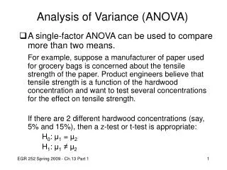
2. One-Way Analysis of Variance • The simplest case of ANOVA is when a single factor determines the populations being compared. • The Completely Randomized Design (CRD) is the simplest of experimental designs, and it commonly lends itself to ANOVA techniques. A CRD involves either • randomly sampling from each of Ipopulations • having the observations within a single population randomly assigned one of Itreatments.

3. ANOVA • Appropriate Hypothesis:

4. ANOVA • It is a single test which simultaneously tests for any difference among the Ipopulation means, thus it controls the experimentwiseerror rate at α. • Multiple comparison procedures can be used to explore the specific differences in the means if the initial ANOVA shows that differences do exist. • This approach is much better than performing all pairwisecomparisions.

5. Bonferonni Correction • Performing all pairwise comparisons if there are Itreatments will results in an experimentwiseerror rate of • The Bonferonni Correction to get 0.05 as the experimentwise error rate is use 0.05 divided by the number of tests performed as the significance level for each individual test

6. Multiple Comparisons • Multiple comparison procedures can be used to explore the specific differences in the means. • Can be stand-alone procedure or done in conjunction with a statistically significant ANOVA test. • Better approach than performing all pairwise comparisons. • Common methods: Fisher, Duncan, Tukey, SNK, Dunnett

7. ANOVA • Assumptions • Independent Random Samples • Normally distributed populations with means mi and common variance s2. • ANOVA is robust to these assumptions • Proper sampling takes care of 1st assumption • Normality can be checked with residual analysis, either an appropriate plot or a normality test • Common variance can be checked with a Bartlett F test

8. ANOVA (balanced) • Mean square for treatments (between)

9. ANOVA (balanced) • Mean square for error (within)

10. ANOVA (balanced) • Test Statistic for one-factor ANOVA is • has an F distribution with numerator degrees of freedom I-1 and denominator degrees of freedom I(J-1) = n- I.

11. Interpreting the ANOVA F If H0 is true, both MS are unbiased whereas when H0 is false, E(MSTr) tends to overestimate s2, so H0 is rejected when F is too large.

12. ANOVA Table • The total variation is partitioned into that due to treatment and error, so the DF and SS for Treatment and Error sum to the Total.

13. ANOVA (unbalanced) • For an unbalanced design, the Total Sum of Square is: where df = n-1

14. ANOVA (unbalanced) • Mean square for treatments (between) • Where df = I-1, so

15. ANOVA (unbalanced) • Mean square for Error (within) where df = n-I, so

16. Multiple Comparisons • Procedures that allow for comparisons of individual pairs or combinations of means. • Post hoc procedures are determined after the data is collected and vary greatly in how well they control the experimentwise error rate.

17. Fisher’s LSD • Fisher’s Least Significant Difference is powerful, but does not control experimentwise error rate • Reject H0 that mi=mk if

18. Tukey’s HSD • Tukey’sHonest Significant Difference is less powerful, but has full control over the experimentwise error rate • Reject H0 that mi=mk if Note: Q is value from the studentized range distribution in Table A10.