Efficient Multilevel Optimization Techniques for Various Problem Types
540 likes | 560 Views
Explore the benefits of multilevel optimization, including linear running time and easier problem-solving with good coarsening techniques. Learn about different relaxation methods, such as strict minimization and steepest descent. Dive into specific cases like Ising models and numerical derivatives using Newton's Method.

Efficient Multilevel Optimization Techniques for Various Problem Types
E N D
Presentation Transcript
Easy Optimization Problems, Relaxation,Local Processingfor a single variable
The advantages of multileveling • Linear running time • Provided a “good coarsening” is performed: 1.The number of variables is reduced in such a way that preserves the essence (skeleton) of the graph => an easier problem 2.Enables processing in different scales, moves which are not likely to happen systematically in a “flat” approach • A better GLOBAL solver
General 1D Arrangement Problems A graph G(v,E) aij
i j xi xj General 1D Arrangement Problems From the graph E(x)=i jai j| xi -xj |p xi = vi /2 + k:p(k)<p(i) vk aij aij To the arrangement
The complexity of pointwise relaxation for P=2 Go over all variables in lexicographic order, put xi at the weighted average location of its graph neighbors Problem: Does not preserve the volume demands! Reinforce volume demands at the end of each sweep • If the reinforcement is done after every variable, the complexity will be quadratic and not linear ! • Sorting of xi is O(nlogn), however, usually logn<C, where C is the constant of the linear complexity • If the ‘sort’ is too slow, use bucketing instead
Different types of relaxation • Variable by variable relaxation – strict minimization • Changing a small subset of variables simultaneously – Window strict minimization relaxation • Stochastic relaxation – may increase the energy – should be followed by strict minimization
Variable by variable strict unconstrained minimization • Discrete (combinatorial) case : Ising model
Exc#1: 2D Ising spins exercise • Minimize • Periodic boundary condition • Initialize randomly: with probability .5 • Go over the grid in lexicographic order, for each spin choose 1 or -1 whichever minimizes the energy (choose with probability ½ when the two possibilities have the same energy) until no changes are observed. 2. Repeat 3 times for each of the 4 possibilities of (h1,h2). 3. Is the global minimum achievable? 4. What local minima do you observe?
Variable by variable strict unconstrained minimization • Discrete (combinatorial) case : Ising model • Quadratic case : P=2 • General functional : P=1 , P>2
Exc#2: Pointwise relaxation for P=1 • Minimize • Pick a variable , fix all at • Minimize • Find the optimal location for
Pointwise relaxation for P=6 • Minimize • Pick a variable , fix all at • Minimize • Find the roots (zeros) of
Variable by variable strict unconstrained minimization • Discrete (combinatorial) case : Ising model • Quadratic case : P=2 • General functional : P=1 , P>2 • Newton’s Method
Newton’s Method (Newton-Raphson) • Geometry • Taylor expansion Starting close enough to the root results with a very fast convergence • What is “close enough”? • May even diverge or oscillate • Verify local reduction in E
Variable by variable strict unconstrained minimization • Discrete (combinatorial) case : Ising model • Quadratic case : P=2 • General functional : P=1 , P>2 • Newton’s Method • Verify local reduction in E • Numerical derivatives
Numerical derivatives • Newton’s Method : • Calculate numerically
Variable by variable strict unconstrained minimization • Discrete (combinatorial) case : Ising model • Quadratic case : P=2 • General functional : P=1 , P>2 • Newton’s Method • Verify local reduction in E • Numerical derivatives • Steepest descent
Steepest descent • Level sets
Steepest descent • Level sets E(x,y)=x2+y2
Steepest descent • Level sets E(x,y)=x2+y2 c2 c1 c1 <c2
Steepest descent • Level sets • The gradient at a point is perpendicular to the level set and is directed towards the maximal rate of increase in the energy • Vector field of gradients
Steepest descent The vector field of the gradient of E(x,y)=x2+y2 At every point it is perpendicular to the level set c2 c1 c1 <c2
Steepest descent • Level sets • The gradient at a point is perpendicular to the level set and is directed towards the maximal rate of increase in the energy • Vector field of gradients => Choose the opposite direction of the gradient as the direction for maximal decrease of the energy How much should you go in this direction?
Variable by variable strict unconstrained minimization • Discrete (combinatorial) case : Ising model • Quadratic case : P=2 • General functional : P=1 , P>2 • Newton’s Method • Verify local reduction in E • Numerical derivatives • Steepest descent • Line search
Line search • Starting at some • Minimize along • Exact minimization: solve • Guess an and use backtracking • Quadratic approximation: Choose , then , draw a parabola through the 3 points and find its minimum • Verify local reduction in E • If not - choose the available minimum
Exc#3: Steepest descent exercise For at Find the steepest descent direction Compare its analytical and numerical calculations Choose 2 small steps in this direction Draw a parabola through the 3 points Find the minimum of the parabola Verify reduction in the energy Find a step that increases the energy
An example of a single node relaxation for the placement problem
The placement problem Given a hypergraph: 1. A list of nodes each with its length and pins’ location 2. A list of lists of subsets of nodes - hyperedges
The placement problem Given a hypergraph: 1. A list of nodes each with its length and pins’ location 2. A list of lists of subsets of nodes - hyperedges • Minimize the sum of all wires approximated by the half Bounding Box of each hyperedge
Pins’ locations Bounding Box The bounding box
The placement problem Given a hypergraph: 1. A list of nodes each with its length and pins’ location 2. A list of lists of subsets of nodes - hyperedges • Minimize the sum of all wires approximated by the half Bounding Box of each hyperedge • Approximate the hypergraph by a graph and the Bounding Box by a quadratic functional
From hypergraph to graph Add avirtual node at the center of mass of the nodes belonging to an hyperedge
From hypergraph to graph Add avirtual node at x0 , the center of mass of the nodes The resulting graph is x1 x4 x0=(x1 +x2 +x3 +x4) /4 x3 x2 E(x)=Si(xi - x0)2 , i=1,…,4 By eliminating x0 : E(x)=Sij(xi - xj)2/4 , i,j=1,…,4
x1 x4 x3 x2 From hypergraph to graph A hyperedge with n nodes contributes n(n-1)/2 quadratic terms with weight 1/n to E(x) Creates a clique of connections E(x)=Sij(xi - xj)2/4 , i,j=1,…,4
The placement problem Given a hypergraph: 1. A list of nodes each with its length and pins’ location 2. A list of lists of subsets of nodes - hyperedges • Minimize the sum of all wires approximated by the half Bounding Box of each hyperedge • Approximate the hypergraph by a graph and the Bounding Box by a quadratic function The placement has 2 phases: global and detailed • Use the original definition towards the detailed
Approximations for the placement problem • Given a hypergraph => translate it to a graph • The nodes are now connected at their center of mass (not at the pins) with straight lines (not rectilinear connections) • The used energy function is quadratic (not the bounding box) • Towards the end of the global placement and definitely at the (discrete) detailed placement use the original definition of the problem not the approximations
Data structure For each node in the graph keep • A list of all the graph’s neighbors: for each neighbor keep a pair of index and weight • … • … • Its current placement • The unique square in the grid the node belongs to For each square in the grid keep • A list of all the nodes which are mostly within • Defines thecurrent physical neighborhood
The augmentedE(xi,yi) to be minimized For node i, fix all other nodes at their current and minimize the augmented functional ----------- ---------------------------------- -------------------- where jare the nodes in the 3x3window of squaresaround the square which includes i
The augmentedE(xi,yi) to be minimized For node i, fix all other nodes at their current and minimize the augmented functional ----------- ---------------------------------- -------------------- where jare the nodes in the 3x3window of squaresaround the square which includes i • How can the “steepest descent direction” be found?
The augmentedE(xi,yi) to be minimized For node i, fix all other nodes at their current and minimize the augmented functional ----------- ---------------------------------- -------------------- where jare the nodes in the 3x3window of squaresaround the square which includes i • How can the “steepest descent direction” be found? • Use numerical “discrete derivatives” • For simplicity calculate each direction separately! • This is anumerical discrete line search minimization