Download
1 / 38
380 likes | 641 Views
6th PEP General Meeting Lima, Peru, June 9-16, 2007. Tax Changes in Argentina: A General Equilibrium Analysis . Martín Cicowiez, Javier Alejo, Luciano Di Gresia, Sergio Olivieri and Ana Pacheco. Centro de Estudios Distributivos, Laborales y Sociales (CEDLAS) www.depeco.econo.unlp.edu.ar/cedlas.

E N D
6th PEP General MeetingLima, Peru, June 9-16, 2007 Tax Changes in Argentina:A General Equilibrium Analysis Martín Cicowiez, Javier Alejo, Luciano Di Gresia, Sergio Olivieri and Ana Pacheco Centro de Estudios Distributivos, Laborales y Sociales (CEDLAS)www.depeco.econo.unlp.edu.ar/cedlas
Outline • Introduction • Data • Methodology • Results
Motivation • The 2001/02 crisis implied a fall in the GDP of more than 15%. The economy has strongly recovered since then, reaching levels of activity similar to those in the 1990s. • The exports and financial transactions taxes that were introduced during the 2001/02 crises are considered as the most distortive in the Argentine tax system by many observers. • Our objective is to evaluate some of the tax changes that are being proposed by different observers. • In this preliminary report we are not trying to “optimize” the Argentine tax structure.
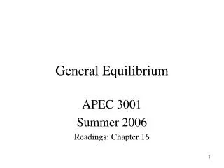
Poverty 1974-2006Share of population below the official moderate poverty line (%) Source: Own estimates from microdata of the EPH (<www.depeco.econo.unlp.edu.ar/cedlas>)
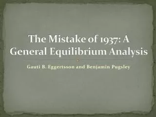
Inequality 1974-2005Gini coefficient household per capita income Source: Own estimates from microdata of the EPH (<www.depeco.econo.unlp.edu.ar/cedlas>)
Proposed Tax Changes • Recently proposed tax changes by different observers as academics, businessmen, private organizations, and policy makers: • reduction in the export tax; • reduction in the financial transactions tax; • reduction in the value added tax on food and beverages; • reduction in the sub-national turnover tax on agriculture and manufactures; • increase in the income tax;
Why Dynamic CGE-Microsimulation? • The (sequential) dynamic CGE model captures the economy-wide and growth effects of tax changes. • The microsimulation model, in turn, allows for an assessment of the poverty and inequality impact of tax changes.
Data Sources: CGE Model • A 2005 SAM was built for this project, • based on 1997 IO tables (latest available) but updated to 2005 using different data sources (national account, government budget data, among others) • three labor categories: unskilled; semi-skilled; and skilled • 25 activities and commodities: 4 agr; 13 mnf; and 8 svc • nine different tax instruments • one household • The SAM is combined with other data in order to calibrate the CGE model, • number of workers in each sector • elasticities -- sensitivity analysis • growth projections for GDP, population, and labor force by skill level • unemployment by skill level
Data Sources: Microsimulation Model • We use the Encuesta Permanente de Hogares (EPH), the main household survey in Argentina. • The EPH gathers information on individual sociodemographic characteristics, employment status, hours of work, wages, incomes, type of job, education, and migration status. • There is no alternative to the use of the (urban) EPH. No attempt was made to reconcile the household survey data with the national accounts. We focus on labor income.
The CGE Model • Recursive dynamic but can be solved in multi-pass or one-pass -- possibility of adding forward-looking behavior. • Labor is perfectly mobile between sectors while capital is sector-specific. • Endogenous labor supply and unemployment with a downward rigid real wage for each type of labor. The minimum real wage for each skill level varies with the following determinants (van der Mensbrugghe, 2005): • the unemployment rate as in a wage curve; • real living standards captured by the household consumption per capita; and • average real factor returns (price of value added).
The CGE Model • Stone-Geary utility function that allows for commodity-specific income elasticities; labor-leisure choice. • Commodities are differentiated according to their country of origin (Armington, 1969). • Quantitative restrictions on exports of agri-food products that generate quota rents. • The behavior of the government income and expenditure depends on the selected closure rule. • The behavior of aggregate real investment depends on the selected closure rule for the savings-investment balance.
The CGE Model • Between periods updates in: sectoral capital stocks; labor force by skill level; minimum consumption; transfers between institutions. • Between periods the new capital (i.e., investment) is distributed between sectors according to their relative rate of return for capital and initial share in total capital stock. • Transfers between institutions grow exogenously at the same rate as GDP in the baseline scenario. • Differences between the simulation scenarios (i.e., policy-influenced) to the baseline are interpreted as the economy-wide impact of tax changes.
The CGE Model: Value Added Tax • The modeling of the value added tax incorporates rebates for intermediate inputs and investment purchases (Go et al., 2005). With this treatment, there is no cascading effect on prices of taxes on intermediate goods. • All transactions are taxed at a fixed proportional rate regardless of whether they are final or intermediate transactions. Firms can deduct taxes paid on intermediate inputs. • Import sales are subject to a VAT while export sales are not.
The Microsimulation Model • At the microsimulation level we produce a counterfactual household income distribution for each time period of the simulation. • The microsimulation involves, in each time period, the following eight steps: • households reweighing to reflect population growth; • labor supply adjustment; • unemployment rate adjustment; • sectoral employment change; • relative wage changes; • average wage changes; • changes in the skill composition of the labor force; and • price changes.
The Microsimulation Model • Every step of the microsimulation produces a counterfactual labor income for each worker. This new labor income is used to compute a counterfactual household income. • We use econometric estimations to compute counterfactual wages for those individuals that change their characteristics in a simulation. • The last step involves a change in the poverty line in order to reflect the price movement of different goods. • The non-labor income is considered constant throughout the whole simulation period.
Macro-Micro Interaction • The two methodologies are used in a sequential fashion (i.e., top-down approach). • The link between both modeling stages is made trough the mapping of changes in wages and employment, and product prices from the CGE to the microsimulation. • We do not need to assure complete consistency between the data sets used at the two modeling stages. Only deviations from the benchmark are transmitted from the CGE model to the microsimulation model.
Scenarios • 1. BASE, business-as-usual scenario; reflects the evolution of the economy in the absence of shocks. • 2. RETENC, 20% yearly reduction starting in year 2008 of the export tax that was introduced during the 2001/02 economic crisis. • 3. IVAALI, 55% reduction in 2008 of the VAT on food; has been proposed to compensate the increase in the domestic price of food that is expected as a consequence of RETENC. • 4. FINANC, 15% in 2008, 20% in 2009, and 25% in 2010 reduction in the financial transactions tax that was also introduced during the 2001/02 economic crisis. • 5. GANANC1-2, in order to compensate the loss of tax revenues induced by the previous tax changes, some analyst have proposed an increase in the income tax in 2008; two variants: 1) 15%; and 2) 20%.
Scenarios • 6. PAQUET1-2, combines all the previous tax changes; two variants: 1) 15% increase in the income tax; and 2) 20% increase in the income tax. • 7. PAQUET1-CHGCLOS, in order to test the sensitivity of some results to the selected closure rule, we run the previous scenario but fixing the government consumption and flexing the ratio between government savings and GDP at market prices. • 8. TOT, 2.5% yearly decrease in the price of exports starting in 2008. • 9. PAQUET1-TOT, combines scenarios TOT and PAQUET1 in order to analyze if the proposed tax changes are useful to isolate the economy from external shocks.
Closure Rule Baseline • Calibration run (i.e., endogenous TFP and exogenous GDP) to impose a GDP growth rate in the baseline scenario. • Fix shares of government consumption, investment, and private consumption in absorption. • Fix foreign savings and flexible real exchange rate to equilibrate the current account of the BOP. • Flexible government savings. • All tax rates are exogenously imposed. • Quantitative restrictions on exports of agri-food products for the period 2006-2007.
Closure Rule Simulations(changes w.r.t. baseline) • Exogenous TFP and endogenous GDP. • Flexible government consumption. • Fix (at BaU values) ratio between government savings and GDP at market prices to assure fiscal solvency -- sensitivity analysis. • Flexible investment and fix (at BaU values) savings rates for domestic non-government institutions. • Fix foreign savings and flexible real exchange rate to equilibrate the current account of the BOP.
Sensitivity Analysis w.r.t. Government Closure RuleGovernment Savings / GDP (%)
Results • The reduction of distortive taxes generates efficiency gains that translate into a higher GDP. • As expected, the reduction in the export tax increases exports and domestic prices. Specifically, the price of food increases relative to the baseline having a negative impact on poverty by moving the poverty line. • The reduction in the VAT for food products compensates the increase in domestic prices generated by the reduction in export taxes.
Results • The closure rule that we are using for our simulations generates a decrease in government consumption as a consequence of the decrease in tax revenue. However, the ratio of tax revenue to GDP reaches historical levels. • When the government closure rule is changed, the proposed tax changes (see PAQUET1) generate a decrease in fiscal solvency and a crowding out of private investment that hurts economic growth.
Results • Poverty decreases in the PAQUET1 scenario mainly as consequence of the decrease in unemployment and the increase in the average wage. • Notice that we do not consider the positive effect that government consumption may have on productivity (e.g., by increasing infrastructure).
Sensitivity Analysis w.r.t. Elasticities Values • The methodology used is based on Harrison and Vinod (1992). The procedure can be summarized in the following steps: • i) randomly select a set of parameters; • ii) solve the model; • iii) store the results; • iv) repeat steps (i) – (iii) several times; and • v) construct confidence intervals for some results. • For this preliminary report, the model was solved only 40 times.
Sensitivity Analysis w.r.t. Elasticities ValuesUnemployment Rate