Download
1 / 34
340 likes | 433 Views
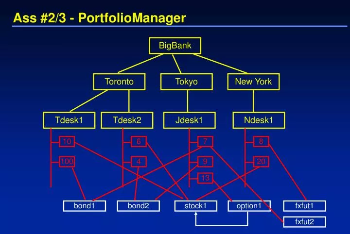
Ass #2/3 - PortfolioManager. BigBank. Toronto. Tokyo. New York. Tdesk1. Tdesk2. Jdesk1. Ndesk1. 10. 6. 7. 8. 100. 4. 9. 20. 13. bond1. bond2. stock1. option1. fxfut1. fxfut2. PortfolioMangaer. % java PortfolioManager infile mark-to-market: $230,942,340

E N D
Ass #2/3 - PortfolioManager BigBank Toronto Tokyo New York Tdesk1 Tdesk2 Jdesk1 Ndesk1 10 6 7 8 100 4 9 20 13 bond1 bond2 stock1 option1 fxfut1 fxfut2
PortfolioMangaer % java PortfolioManager infile mark-to-market: $230,942,340 CADdown: -$3,456,333 Irdown: +$2,456 … instruments portfolio/positions market data scenarios ASCII, XML Zero coupon bonds FX futures Equities European equity call options
Interest Rates - Pricing a Bond Zero Coupon Bond • Face Value: $1000 • Matures: April 19, 2001 • Interest: 5% simple $1050 6 months 19/10/2000 19/04/2001 What would you pay for it? $?,???
$(1.07xP) T T + 6mo. $P Interest Rates - Relative Pricing It depends on what other investments are available. Assume only other investment is a US T-Bill returning 7% each half-year.
$(1.07xP) T T + 6mo. $P Interest Rates - Pricing the First Coupon $1050 Alternate investment. 19/10/2000 19/04/2000 $?? $1050 = 1.07 x P P = $981.31 Supply and Demand will bring prices in-line
Interest Rates - Adding More Realism • Actually, • T-Bills are priced by the market like anything else. • There are alternative investments at all sorts of maturities out to 30 years.
Interest Rates - The Spot Zero Curve The “spot zero curve” captures these rates of return in one concise curve. Gives YTM (yield-to-maturity) for non coupon bearing bonds of various maturities. Better to use a concept called “discount factors”
Interest Rates - Units • Discount Factors • converts future dollars to present dollars • Can express equivalently as interest rates which are considerably more intuitive. Say 5yr. discount factor is 0.50835 Bond worth $1000 five years from now costs $508.35 today. Can express YTM of bond in units of annualised interest compounded annually. Can also express in units of annualised interest compounded semi-annually. All the same!
98/01/01 98/06/01 99/01/01 99/06/01 00/01/01 00/06/01 01/01/01 01/06/01 02/01/01 $1000 02/06/01 03/01/01 xY xY xY xY xY xY xY xY xY xY $508.35 Interest Rates - Compounded Units x 0.50835 508.35 x Y10 = $1000 Y = 1.07 YTM = 7% semi-annual, semi-annually compounded YTM = 14% annualised, semi-annually compounded
Time in days = Time in years Daycount Interest Rates - Daycount Basis Glossed over issue of units of time. Actually, all units are in days, although they seem to be quoted in years! Missing bit of information is the “daycount basis”. • Examples of daycount bases: ACT/360, ACT/365, ACT/ACT
$50 98/01/01 98/06/01 $46.73 Interest Rates - Years in Daycount of Bond • Years between 98/01/01 and 98/06/01are computed as follows: • Days between = 31 + 28 + 31 + 30 + 31 + 30 = 181 • For a ACT/360 daycount, Time in years = 181/360 = 0.50278 • For a ACT/365 daycount, Time in years = 181/365 = 0.49589 • For a ACT/ACT daycount, Time in years = 181/365 = 0.49589 • (if 1998 was a leap year), Time in years = 182/366 = 0.49727
98/01/01 98/06/01 99/01/01 99/06/01 00/01/01 00/06/01 01/01/01 01/06/01 02/01/01 $1000 02/06/01 03/01/01 2*days/360 ( ) 1 + YTM5 $508.35 1 2 x $1000 $508.38 = Interest Rates - Converting using Daycount x 0.50835 days = 365 + 365 + 366 + 365 + 365 = 1826 ACT/360 daycount basis annualised rates w/ semi-annual compounding
Interest Rates - Same Rate, Different Units YTM annualised rates, semi-annually compounded, ACT/360 daycount 13.793% annualised rates, semi-annually compounded, ACT/365 daycount 13.991% annualised rates, semi-annually compounded, ACT/ACT daycount 13.999% annualised rates, annually compounded, ACT/ACT daycount 14.489% annualised rates, daily compounded, ACT/365 daycount 13.526% annualised rates, continuously compounded, ACT/365 daycount 13.523%
m*days/365 ( ) 1 + YTM5 1 m x $1000 $508.38 = Interest Rates - Continuous Compounding In the limit as ‘m’ (number of compounding periods in a year) goes to infinity: e-YTM x days/365 $508.38 = x $1000 YTM = -ln(508.38/1000)*365/1826 = 13.523% cont. ACT/365
Interest Rates - Bond Pricing w/ a Zero Curve $1,050 Bond pricing using a “real” spot zero curve 98/01/01 03/01/01 Units are annualised rates, continuously compounded, on an ACT/365 daycount basis P = $1050 x e- 0.06 x 5.03 P = $776.46
Interest Rates - Parity • Each distinct currency has its own zero curve. • No reason borrowing in USD should be the same rate as borrowing in CAD. USD 1yr. rate = 10% ANNU ACT/ACT CAD 1yr. rate = 5% ANNU ACT/ACT • Q. Why not convert into USD and invest there? A. Because exchange rates could move in 1yr. and kill you. • But, by using FX Futures contracts, I can lock in a rate today and know exactly what the exchange rate will be in 1yr.’s time.
Interest Rates - Parity • This leads to a relationship between • the CAD-USD spot fx rate, • the USD 1yr. spot IR rate, • the CAD 1yr. spot IR rate, • the CAD-USD 1yr. forward fx rate. • If this relationship is broken, arbitrageurs working at large banks will trade and make instantaneous risk-free profits. • Forces of supply and demand will force the prices back into alignment.
$137 CAD $143.85 CAD $110 USD $100 USD Interest Rates - Parity 1yr. rate = 5% ANNU ACT/ACT Borrow in Canada spot fx = 1.37 CAD/USD 1yr. forward fx must be = 1.31 CAD/USD If Not... Lend in U.S. 1yr. rate = 10% ANNU ACT/ACT
Interest Rates - IR Parity Arbitrage Say 1yr. future fx rate was 1.37 and not 1.31. • Borrow $100 CAD at 5% (owe $105 CAD in 1yr.’s time) • Buy $4.55 CAD worth of candy bars. • Convert $95.45 CAD at 1.37 to $69.67 USD • Loan $69.67 USD at 10% • Enter into 1 yr. fx forward contract at 1.37 CAD/USD • In 1 yr.’s time • Get back $76.64 USD • Use forward contract to convert to $105 CAD at 1.37 CAD/USD • Pay back $105 CAD dept in its entirety • Net result: Ahead 4 candy bars! No risk taken!
+$1,000 +$2,000 50% 50% -$1,000 -$???? 50% 50% +$1,000 $0 Option Pricing • Deals with the valuation of risky securities. Q. How much would you pay? A. It depends.
Option Pricing - Stock Call Option Call Option • Option to purchase 100 shares of IBM stock • On Feb.17, 1998 • At a strike of $65 per share • Current price is $62 $?? 97/10/22 98/01/17 $?? What would you pay for it?
Option Payout St-X X Stock Price: St Option Pricing - Call Option Payout 100 x (St - X) X = $65 97/10/22 So = $62 $0 98/01/17
X St Time Stock Price + Option Pricing - Computing Option Value S0
Option Pricing - Model of Stock Prices • To compute distribution of stock price in the future, we need a model of how stock prices will change through time. • Model used is geometric Brownian motion.
Option Pricing - Markov Process • A stochastic process where only the current value is relevant for predicting the next value • Past history is not taken into account.
z t Option Pricing - Wiener Process • Also called Brownian motion • Used in Physics to describe the motion of a particle that is subject to a large number of small molecular shocks. dz = n . sqrt(dt) where n is drawn from a standardised normal distribution N(0,1)
Option Pricing - The Generalised Wiener Process dz = n . sqrt(dt) expected drift rate mean of change in x = a.T variance of change in x = b2.T dx = a.dt + b.dz variance rate where a and b are constants. x = a.t x t T
Option Pricing - Ito Process dz = n . sqrt(dt) dx = a(x,t).dt + b(x,t).dz where a and b are functions of x and t.
Option Pricing - Stock Process S0=60, m=14%, s=20% dS/S = m.dt + s.dz dS = S.m.dt + S.s.dz constant rate of return drift constant rate of return variance T
S.u5 S.u4.d S.u S.u3.d2 p S 1-p S.u2.d3 S.d S.u.d4 S.d5 Option Pricing - Lattices Can model this process as a lattice on stock prices. u = es.sqrt(dt) dt d = 1/u p = (em.dt - d)/(u-d)
Option Pricing - Example Lattice S0=100, m=12%, s=30% $127.1 (p = 0.076) $119.7 $112.7 $112.7 (p = 0.275) $106.2 $106.2 $100 0.525 $100 $100 (p = 0.373) $94.2 $94.2 0.475 $88.7 $88.7 (p = 0.225) $83.6 dt = 0.04 yr. $78.7 (p = 0.051)
$127.1 $17.1 (p = 0.076) $119.7 $112.7 $112.7 $2.7 (p = 0.275) X = $110 $100 $106.2 0.525 $106.2 $100 $100 $0 (p = 0.373) $94.2 $94.2 0.475 $88.7 $88.7 $0 (p = 0.225) $83.6 dt = 0.04 yr. $78.7 $0 (p = 0.051) Option Pricing - Pricing an Option S0=100, m=12%, s=30% Discount back! Option expected value = 0.076 x $17.10 + 0.275 x $2.70 = $2.04
Option-Pricing - Black-Scholes In the limit as dt ®0, can derive a closed-form solution for the expected value of a European option. Black-Scholes equation. Nobel Prize c = S.N(d1) - X.e-r.(T-t).N(d2) d2 = d1 - s.sqrt(T-t) d1 = (ln(S/X) + (r+s2/2).(T-t)) / s.sqrt(T-t)