Download
1 / 9
90 likes | 204 Views
Traffic Congestion and Congestion Pricing- Time independent and time dependent analysis. Congestion pricing in time independent model. Assumption: Consider one origin and one destination connected by a single road. Individuals make trips alone in identical vehicles.

E N D
Traffic Congestion andCongestion Pricing- Time independent and time dependent analysis
Congestion pricing in time independent model Assumption: • Consider one origin and one destination connected by a single road. • Individuals make trips alone in identical vehicles. • Traffic flows, speeds and densities are uniform along the road and independent of time.
Time independent traffic congestion model: The horizontal axis depicts traffic flow or volume: the rate at which trips are initiated and completed. The verticalaxis depicts the price or ‘generalized cost’ of a trip —which includes vehicle operating costs, the time costs of travel, and any toll. At low volumes vehicles can travel at the free flow speed, and the trip cost curve, C(q), is constant at the free flow cost Cff. At higher volumes congestion develops, speed falls, and C(q) slopes upwards. If flow is interpreted to be the quantity of trips “demanded” per unit of time, then a demand curve p(q) can be added to Figure 1 to obtain a supply-demand diagram.
The demandcurve is assumed to slope downwards to reflect the fact that, as for most commodities, the number of trips people want to make decreases with the price. The unregulated ‘no-toll’ equilibrium occurs at the intersection of C(q) and p(q), resulting in an equilibrium flow of qnand an equilibrium price of Cn. ‘external benefits’ of road use are not likely to be significant, p(q) specifies both the private and the marginal social benefit of travel. Total social benefits can thus be measured by the area under p(q). Analogously, C(q) measures the cost to the traveler of taking a trip. If external travel costs other than congestion, such as accidents and air pollution, are ignored, then C(q) measures the average social cost of a trip. The total social cost of q trips is then TC(q) = C(q) . q , and the marginal social cost of an additional trip is MC(q) =dTC(q)/dq = C(q)+q .dC(q)/dq . cn qn
The social optimal is found in Figure 1 at the intersection of MC(q) and p(q) , where the marginal willingness to pay for trips is MCo and the number of trips, qo, is less than in the unregulated equilibrium. The optimum can be supported as an equilibrium if travelers are forced to pay a total price of MCo. Because the price of a trip is the sum of the individual’s physical travel cost and the toll, the requisite toll is,ᶯ = MC(q0) – C(q0)= q0 .dC(q0)/dq where q0 . dC(q0)/dq is the marginal congestion cost imposed by a traveler on others. This toll is known as a ‘Pigouvian’ tax, after Pigou in 1920.