Download
1 / 13
140 likes | 298 Views
Sparse matrix computations. Dave O’Hallaron Intel Research Pittsburgh Sept 2007. element. node. t. mesh. simulation results. Galerkin discretization. FEM solver. Animation. Visualization Model. Mathematical Model. Computer Model. Numerical Model. Physical Model. Physical

E N D
Sparse matrix computations Dave O’Hallaron Intel Research Pittsburgh Sept 2007
element node t mesh simulation results Galerkin discretization FEM solver Animation Visualization Model Mathematical Model Computer Model Numerical Model Physical Model Physical System Wave propagation equation Material property model Earthquake ground motion Scientific Computing Process
t Scientific Computing Workflow Physical model Mesh Simulation results Solver Mesh generation Visuali- zation Mesh
David O’Hallaron (CMU CS and ECE) Jacobo Bielak (CMU CivE)
1994 Northridge Quake Simulation 20 seconds of an aftershock from the Jan 17, 1994 Northridge quake in San Fernando Valley of Southern California.
Teora, Italy 1980
lat. 34.38 long. -118.16 epicenter lat. 34.32 long. -118.48 x San Fernando Valley lat. 34.08 long. -118.75 San Fernando Valley
San Fernando Valley (Top View) Hard rock epicenter x Soft soil
San Fernando Valley (Side View) Soft soil Hard rock
nodes element Partitioned Unstructured Mesh
The disp vector records the displacements of each mesh node during last three timesteps Quake solver code NODEVECTOR3 disp[3], M, C, M23; MATRIX3 K; /* matrix and vector assembly */ FORELEM(i) { ... } /* time integration loop */ for (iter = 1; iter <= timesteps; iter++) { SMVP(K, disp[dispt], disp[disptplus]); disp[disptplus] *= - IP.dt * IP.dt; disp[disptplus] += 2.0 * M * disp[dispt] - (M - IP.dt / 2.0 * C) * disp[disptminus] - ...); disp[disptplus] = disp[disptplus] / (M + IP.dt / 2.0 * C); i = disptminus; disptminus = dispt; dispt = disptplus; disptplus = i; } K is the adjacency matrix of the mesh, a labeled undirected graph 90% of time spent in sparse matrix vector product (SMVP) kernel