Download
1 / 15
150 likes | 261 Views
Lecture Objectives:. Discuss HW3 Introduce alternative conduction equation solution method Present a commercial software eQUEST and define basic modeling steps. Top view. Homework 3 (Similar to HW2, but unsteady, and more realistic). Glass. T north_oi. T north_i.

E N D
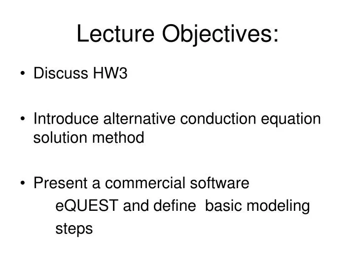
Lecture Objectives: • Discuss HW3 • Introduce alternative conduction equation solution method • Present a commercial software eQUEST and define basic modeling steps
Top view Homework 3 (Similar to HW2, but unsteady, and more realistic) Glass Tnorth_oi Tnorth_i Tinter_surf ≠ Tair 2.5 m Surface radiation Tair_in 10 m IDIR 10 m Teast_i Idif East North Insulation Teast_o Tair_out Concrete Surface radiation Idif IDIR
Alternative: Response function methods for conduction calculation NOTATION: θ(x,t)=T(x,)
Laplace transformation Laplace transform is given by Where p is a complex number whose real part is positive and large enough to cause the integral to converge.
Principles of Response function methods The basic strategy is to predetermine the response of a system to some unit excitation relating to the boundary conditions anticipated in reality. Reference: JA Clarke http://www.esru.strath.ac.uk/Courseware/Class-16458/ or http://www.hvac.okstate.edu/research/documents/iu_fisher_04.pdf
Response functions • Computationally inexpensive • Accuracy ? • Flexibility ???? What if we want to calculate the moisture transport and we need to know temperature distribution in the wall elements?
Modeling 1) External wall (north) node Qsolar+C1·A(Tsky4 - Tnorth_o4)+ C2·A(Tground4 - Tnorth_o4)+hextA(Tair_out-Tnorth_o)=Ak/(Tnorth_o-Tnorth_in) A- wall area [m2] • - wall thickness [m] k – conductivity [W/mK] - emissivity [0-1] • - absorbance [0-1] • = - for radiative-gray surface, esky=1, eground=0.95 Fij –view (shape) factor [0-1] h – external convection [W/m2K] s – Stefan-Boltzmann constant [5.67 10-8 W/m2K4] Qsolar=asolar·(Idif+IDIR)A C1=esky·esurface_long_wave·s·Fsurf_sky C2=eground·esurface_long_wave·s·Fsurf_ground 2) Internal wall (north) node C3A(Tnorth_in4- Tinternal_surf4)+C4A(Tnorth_in4- Twest_in4)+hintA(Tnorth_in-Tair_in)= =kA(Tnorth_out--Tnorth_in)+Qsolar_to_int_ considered _surf Qsolar_to int surf =portion of transmitted solar radiation that is absorbed by internal surface C3=eniort_in·s·ynorth_in_to_ internal surface for homeworkassume yij = Fijei
Modeling b1T1 + +c1T2+=f(Tair,T1,T2) a2T1+b2T2 + +c2T3+=f(T1 ,T2, T3) a3T2+b3T3+ +c3T4+=f(T2 ,T3 , T4) ……………………………….. a6T5+b6T6+ =f(T5 ,T6 , Tair) Matrix equation M × t = f for each time step M × t = f
Modeling steps • Define the domain • Analyze the most important phenomena and define the most important elements • Discretize the elements and define the connection • Write the energy and mass balance equations • Solve the equations (use numeric methods or solver) • Present the result
eQUEST • Energy simulation software • Free: http://doe2.com/equest/ • Graphical user interface (GUI) that uses DOE2 • Easy to use it • Example of your HW1a • ….