Download
1 / 17
170 likes | 262 Views
Nonlinear modulation of O3 and CO induced by mountain waves in the UTLS region during TREX. Mohamed Moustaoui(1), Alex Mahalov(1), Hector Teitelbaum(2) and Vanda Grubisic (3) (1) Arizona State University (2) Laboratoire de Meteorologie Dynamique, Paris (3) University of Vienna.

E N D
Nonlinear modulation of O3 and CO induced by mountain waves in the UTLS region during TREX Mohamed Moustaoui(1), Alex Mahalov(1), Hector Teitelbaum(2) and Vanda Grubisic (3) (1) Arizona State University (2) Laboratoire de Meteorologie Dynamique, Paris (3) University of Vienna
TREX data used in this study are O3, CO and temperature obtained from NCAR/HIAPER aircraft measurements on March 25, 2006. Topography for the microscale nest (domain 4). The black curve shows the path of the plane. Vertical cross section of eastward wind and potential temperature on 25 Mars 2006. The simulation uses three nested WRF domains (dx =27km, 9km, 3km) and a microscale nest (dx=1km). The microscale nest uses grid refinement in the vertical with increased resolution in the UTLS (dz = 80 m). The parent domain uses data from ECMWF T799L91 for initialization and the boundary conditions.
HIAPER observations Simulations q q O3 O3 q O3 Averaged vertical profile of Ozone as a function of potential temperature calculated from aircraft observations on 03-25-2006.
Potential temperature (black, K), O3 (blue, ppb) and CO (red, ppb) mixing ratio as a function of time (hour) measured by HIAPER aircraft for Leg1. The time is relative to 25 March, 2006 15 UTC. The time reflects the spatial variation along the path of the aircraft
Potential temperature (black, K), O3 (blue, ppb) and CO (red, ppb) mixing ratio as a function of time (hour) measured by HIAPER aircraft for Leg2. The time is relative to 25 March, 2006 15 UTC. The time reflects the spatial variation along the path of the aircraft
Vertical profiles of O3 (blue) and the averaged O3 (black) from the aircraft measurements. CO (red) as a function of potential temperature from the aircraft measurements and the averaged vertical profile (black) of CO
Filtered variations of potential temperature (black), O3 (blue) and the altitude of the aircraft (dashed, km) as a function of time.
Potential temperature (black, K), O3 (blue, ppb) as a function of time measured by HIAPER aircraft for Leg1. The dashed curves are the filtered variations. Potential temperature (black, K), O3 (blue, ppb) as a function of time measured by HIAPER aircraft for Leg1. The dashed curves are the filtered variations.
Potential temperature (black, K), O3 (blue, ppb) as a function of time measured by HIAPER aircraft for Leg2. The dashed curves are the filtered variations. Potential temperature (black, K), O3 (blue, ppb) as a function of time measured by HIAPER aircraft for Leg2. The dashed curves are the filtered variations.
Schematic showing the reversal of correlation seen by the aircraft positive correlation aircraft Negative correlation
Variations of O3 (blue) and reconstructed O3 (red) as a function of time calculated from potential temperature (black) for Leg1. Variations of O3 (blue) and reconstructed O3 (red) as a function of time calculated from potential temperature (black) for Leg1
Variations of O3 (blue) and reconstructed O3 (red) as a function of time calculated from potential temperature (black) for Leg2 Variations of CO (blue) and reconstructed CO (red) as a function of time calculated from potential temperature (black) for Leg2
Vertical profiles of potential temperature as a function of altitude (km) from dropsondes (black-dashed, K); and averaged profiles of potential temperature (black-solid, K), O3 (blue, ppb) and CO (red, ppb). averaged vertical profiles of O3 (blue) and CO (red) as a function of potential temperature.
Variations of potential temperature (black), O3 (blue) and CO (red) as a function of distance (km) simulated for altitude (a) z= 11.64 km and (b) z=12.1 km
Variations of potential temperature (black), O3 (blue) and CO (red) as a function of distance (km) simulated for altitude z=12.1 km in the linear case.
Reconstructed O3 using CAS at 342 K initialized with ozone from HIRDLS measurements. The wind fields used for advection are from ECMWF. The ozone fields are shown at 342K on (a) 23 March, (b) 24 March and (c) 25 March. (d) (e) and (f) are the same as (a), (b) and (c) but at 355 K. The red dot indicates the location of TREX observations 342K 355K
Conclusion • Ozone, CO and potential temperature obtained from aircraft measurements in the UTLS region show fluctuations with modulations in phases and amplitudes. • The phase relation between ozone and potential temperature varies in the horizontal. In some legs, ozone and temperature are positively correlated while in other legs the correlation is negative. • The vertical profile of ozone exhibits decreases within a layer in the lower stratosphere, with positive gradients above and below • The phase and amplitude modulations in ozone, CO and potential temperature are produced by interactions of mountains waves with different wavenumbers