Download
1 / 71
710 likes | 784 Views
SEE1012: Introduction to Electrical Engineering. Week 10: Introduction to important software and tools. 1. Introduction to PSpice 2. MATLAB for Engineering Applications. The materials are extracted from: 1. http:// stuweb.ee.mtu.edu 2. http://www.osc.edu/. Introduction to PSpice.

E N D
SEE1012: Introduction to Electrical Engineering Week 10: Introduction to important software and tools
1. Introduction to PSpice2. MATLAB for Engineering Applications The materials are extracted from: 1. http://stuweb.ee.mtu.edu 2. http://www.osc.edu/
The Origins of SPICE • SPICE developed in the 1970’s • Simulation Program with Integrated Circuit Emphasis • Developed to save money • Simulation of circuits, not physically building • Transistor sizes • Microprocessors vs. 2N2222
This Is Now • New user interface • Graphical circuit diagrams • Variation of simulation parameters with a few clicks
First Look at Capture • First window you will see when you open Capture • Create a new Project • File New Project • This will open a new window
New Project Window • Select a project name • PSpice Lab Simulation • Select a project location • C:\PSpice\{YourName} • Select what type of project • Analog or Mixed A/D • Click OK
Create PSpice Project • This window will open • Select the bottom option • Create a blank project • Click OK
The Project Windows • The Main Project Window • Two other information windows • Session Log Window • Project File Window • Our main window • Schematic 1: Page 1
Place Parts • Place the 5 resistors • Using Place Part • Type ‘R’ in Part Field • Place the Voltage Source • Using Place Part • Type ‘Vdc’ in Part Field • Right click and choose “End Mode”
Rotate and Move Resistors • Click on the resistor • Use ‘Ctrl+R’ to rotate • Repeat for 4 resistors • Move and place the resistors in parallel • Change the values • Double Click on the ‘1k’ and enter ‘4k’ of the parallel resistors
Change the Voltage and Wire • Change DC Voltage • Double Click on ‘0Vdc’ and enter ’16Vdc’ • Now wire the circuit • Using Place Wire • Click on one node, and ‘draw’ to the other and click again • Right click and select “End Mode”
Placing the Ground • Every PSpice circuit must have a ground • Use the icons on the right • 9th icon down • This opens the “Place Ground” window • Select the ‘0/Source’ • Click OK
Simulation Profile • Need to create a simulation profile • PSpice New Simulation Profile • Name the profile • DC Solution • Click OK
Edit the Simulation Profile • Go to the Analysis Tab • Under the Analysis type, choose Bias Point • This is to find the DC solution • Click OK • Ready to Simulate
Running the Simulation • The last step is to RUN the simulation • Do this by selecting PSpice Run • After running the simulation a new window will open • Close this window and return to the Schematic 1: Page 1 window • Use the “V” and “I” (and maybe “W”) icons on the top of the screen • For finding voltages and currents (and power)
Now You Know • With this basic underlying knowledge • Can change • Resistor values • Voltage supply values • Resistor configuration • Can learn • More simulation parameters • More components for simulation
MATLAB’s Appeal • Interactive code development proceeds incrementally; excellent development and rapid prototyping environment • Basic data element is the auto-indexed array • This allows quick solutions to problems that can be formulated in vector or matrix form • Powerful GUI tools • Large collection of toolboxes: collections of topic-related MATLAB functions that extend the core functionality significantly Intro MATLAB
MATLAB Toolboxes Math and Analysis Optimization Requirements Management Interface Statistics Neural Network Symbolic/Extended Math Partial Differential Equations PLS Toolbox Mapping Spline Data Acquisition and Import Data Acquisition Instrument Control Excel Link Portable Graph Object Signal & Image Processing Signal Processing Image Processing Communications Frequency Domain System Identification Higher-Order Spectral Analysis System Identification Wavelet Filter Design Control Design Control System Fuzzy Logic Robust Control μ-Analysis and Synthesis Model Predictive Control Intro MATLAB
Toolboxes, Software, & Links Intro MATLAB
MATLAB System • Language: arrays and matrices, control flow, I/O, data structures, user-defined functions and scripts • Working Environment: editing, variable management, importing and exporting data, debugging, profiling • Graphics system: 2D and 3D data visualization, animation and custom GUI development • Mathematical Functions: basic (sum, sin,…) to advanced (fft, inv, Bessel functions, …) • API: can use MATLAB with C, Fortran, and Java, in either direction Intro MATLAB
Online MATLAB Resources • www.mathworks.com/ • www.mathtools.net/MATLAB • www.math.utah.edu/lab/ms/matlab/matlab.html • www.utexas.edu/its/rc/tutorials/matlab/ • www.math.ufl.edu/help/matlab-tutorial/ • www.indiana.edu/~statmath/math/matlab/links.html • www-h.eng.cam.ac.uk/help/tpl/programs/matlab.html Intro MATLAB
References Mastering MATLAB 7, D. Hanselman and B. Littlefield, Prentice Hall, 2004 Getting Started with MATLAB 7: A Quick Introduction for Scientists and Engineers, R. Pratap, Oxford University Press, 2005. Intro MATLAB
Main MATLAB Interface Intro MATLAB
Some MATLAB Development Windows • Command Window: where you enter commands • Command History: running history of commands which is preserved across MATLAB sessions • Current directory: Default is $matlabroot/work • Workspace: GUI for viewing, loading and saving MATLAB variables • Array Editor: GUI for viewing and/or modifying contents of MATLAB variables (openvarvarname or double-click the array’s name in the Workspace) • Editor/Debugger: text editor, debugger; editor works with file types in addition to .m (MATLAB “m-files”) Intro MATLAB
MATLAB Editor Window Intro MATLAB
MATLAB Help Window (Very Powerful) Intro MATLAB
Command-Line Help: List of MATLAB Topics >> help HELP topics: matlab\general - General purpose commands. matlab\ops - Operators and special characters. matlab\lang - Programming language constructs. matlab\elmat - Elementary matrices and matrix manipulation. matlab\elfun - Elementary math functions. matlab\specfun - Specialized math functions. matlab\matfun - Matrix functions - numerical linear algebra. matlab\datafun - Data analysis and Fourier transforms. matlab\polyfun - Interpolation and polynomials. matlab\funfun - Function functions and ODE solvers. matlab\sparfun - Sparse matrices. matlab\scribe - Annotation and Plot Editing. matlab\graph2d - Two dimensional graphs. matlab\graph3d - Three dimensional graphs. matlab\specgraph - Specialized graphs. matlab\graphics - Handle Graphics. …etc... Intro MATLAB
Command-Line Help: List of Topic Functions >> help matfun Matrix functions - numerical linear algebra. Matrix analysis. norm - Matrix or vector norm. normest - Estimate the matrix 2-norm. rank - Matrix rank. det - Determinant. trace - Sum of diagonal elements. null - Null space. orth - Orthogonalization. rref - Reduced row echelon form. subspace - Angle between two subspaces. …
Command-Line Help: Function Help >> help det DET Determinant. DET(X) is the determinant of the square matrix X. Use COND instead of DET to test for matrix singularity. See also cond. Overloaded functions or methods (ones with the same name in other directories) help laurmat/det.m Reference page in Help browser doc det Intro MATLAB
Keyword Search of Help Entries >> lookfor who newton.m: % inputs: 'x' is the number whose square root we seek testNewton.m: % inputs: 'x' is the number whose square root we seek WHO List current variables. WHOS List current variables, long form. TIMESTWO S-function whose output is two times its input. >> whos Name Size Bytes Class Attributes ans 1x1 8 double fid 1x1 8 double i 1x1 8 double Intro MATLAB
startup.m • Customize MATLAB’s start-up behavior • Create startup.m file and place in: • Windows: $matlabroot\work • UNIX: directory where matlab command is issued Mystartup.m file: addpath e:\download\MatlabMPI\src addpath e:\download\MatlabMPI\examples addpath .\MatMPI format short g format compact eliminates extra blank lines in output Intro MATLAB
Variable Basics >> 16 + 24 ans = 40 >> product = 16 * 23.24 product = 371.84 >> product = 16 *555.24; >> product product = 8883.8 no declarations needed mixed data types semi-colon suppresses output of the calculation’s result Intro MATLAB
Variable Basics >> clear >> product = 2 * 3^3; >> comp_sum = (2 + 3i) + (2 - 3i); >> show_i = i^2; >> save three_things >> clear >> load three_things >> who Your variables are: comp_sum product show_i >> product product = 54 >> show_i show_i = -1 clearremoves all variables; clear x y removes only x and y complex numbers (ior j) require no special handling save/loadare used to retain/restore workspace variables use home to clear screen and put cursor at the top of the screen Intro MATLAB
MATLAB Data The basic data type used in MATLAB is the double precision array • No declarations needed: MATLAB automatically allocates required memory • Resize arrays dynamically • To reuse a variable name, simply use it in the left hand side of an assignment statement • MATLAB displays results in scientific notation • Use File/Preferencesand/or format function to change default • short (5 digits), long (16 digits) • format short g; format compact (my preference) Intro MATLAB
Variables Revisited • Variable names are case sensitive and over-written when re-used • Basic variable class:Auto-Indexed Array • Allows use of entire arrays (scalar, 1-D, 2-D, etc…) as operands • Vectorization:Always usearray operands to get best performance (see next slide) • Terminology: “scalar” (1 x 1 array), “vector” (1 x N array), “matrix” (M x N array) • Special variables/functions:ans, pi, eps, inf, NaN, i, nargin, nargout, varargin, varargout, ... • Commands who (terse output) and whos (verbose output) show variables in Workspace Intro MATLAB
Vectorization Example* >> type fast.m tic; x=0.1:0.001:200; y=besselj(3,x) + log(x); toc; >> fast Elapsed time is 0.551970 seconds. Roughly 31 times faster without use of for loop >> type slow.m tic; x=0.1; for k=1:199901 y(k)=besselj(3,x) + log(x); x=x+0.001; end toc; >> slow Elapsed time is 17.092999 seconds. *times measured on this laptop Intro MATLAB
Matrices: Magic Squares This matrix is called a “magic square” Interestingly, Durer also dated this engraving by placing 15 and 14 side-by-side in the magic square. Intro MATLAB
Durer’s Matrix: Creation » durer1N2row = [16 3 2 13; 5 10 11 8]; » durer3row = [9 6 7 12]; » durer4row = [4 15 14 1]; » durerBy4 = [durer1N2row;durer3row;durer4row]; » durerBy4 durerBy4 = 16 3 2 13 5 10 11 8 9 6 7 12 4 15 14 1 Intro MATLAB
Easier Way... durerBy4 = 16 3 2 13 5 10 11 8 9 6 7 12 4 15 14 1 » durerBy4r2 = [16 3 2 13; 5 10 11 8; 9 6 7 12; 4 15 14 1] durerBy4r2 = 16 3 2 13 5 10 11 8 9 6 7 12 4 15 14 1 Intro MATLAB
Multidimensional Arrays >> r = randn(2,3,4) % create a 3 dimensional array filled with normally distributed random numbers r(:,:,1) = -0.6918 1.2540 -1.4410 0.8580 -1.5937 0.5711 r(:,:,2) = -0.3999 0.8156 1.2902 0.6900 0.7119 0.6686 r(:,:,3) = 1.1908 -0.0198 -1.6041 -1.2025 -0.1567 0.2573 r(:,:,4) = -1.0565 -0.8051 0.2193 1.4151 0.5287 -0.9219 “%” sign precedes comments, MATLAB ignores the rest of the line randn(2,3,4): 3 dimensions, filled with normally distributed random numbers Intro MATLAB
Character Strings >> hi = ' hello'; >> class = 'MATLAB'; >> hi hi = hello >> class class = MATLAB >> greetings = [hi class] greetings = helloMATLAB >> vgreetings = [hi;class] vgreetings = hello MATLAB concatenation with blank or with “,” semi-colon: join vertically Intro MATLAB
Character Strings as Arrays >> greetings greetings = helloMATLAB >> vgreetings = [hi;class] vgreetings = hello MATLAB >> hi = 'hello' hi = hello >> vgreetings = [hi;class] ??? Error using ==> vertcat CAT arguments dimensions are not consistent. note deleted space at beginning of word; results in error Intro MATLAB
String Functions yo = Hello Class >> ischar(yo) ans = 1 >> strcmp(yo,yo) ans = 1 returns 1 if argument is a character array and 0 otherwise returns 1 if string arguments are the same and 0 otherwise; strcmpi ignores case Intro MATLAB
Set Functions Arrays are ordered sets: >> a = [1 2 3 4 5] a = 1 2 3 4 5 >> b = [3 4 5 6 7] b = 3 4 5 6 7 >> isequal(a,b) ans = 0 >> ismember(a,b) ans = 0 0 1 1 1 returns true (1) if arrays are the same size and have the same values returns 1 where a is in b and 0 otherwise Intro MATLAB
Matrix Operations >> durer = [16 3 2 13; 5 10 11 8; 9 6 7 12; 4 15 14 1] durer = 16 3 2 13 5 10 11 8 9 6 7 12 4 15 14 1 >> % durer's matrix is "magic" in that all rows, columns, >> % and main diagonals sum to the same number >> column_sum = sum(durer) % MATLAB operates column-wise column_sum = 34 34 34 34 MATLAB also has magic(N) (N > 2) function Intro MATLAB