Download
1 / 54
540 likes | 633 Views
This paper explores the motivation and challenges of translating MATLAB programs to X10 for high-performance computing. It discusses the technical challenges and solutions, including efficient compilation of arrays and concurrency controls. The use of X10's advanced features and the optimization of array indexing are key focuses. The paper also introduces concurrency constructs in MATLAB, such as async and finish, and outlines strategies for parallelizing vector instructions for optimal performance.

E N D
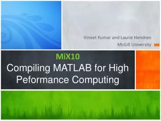
Vineet Kumar and Laurie Hendren McGill University MiX10Compiling MATLAB for High Peformance Computing
1 Why?Whynot ! motivation and challenges
Why MATLAB to X10? I wish I could make better use of that super computer ! I wish my program could run faster ! What do I do about all the programs that are already written ? I wish I had time to learn that cool new language I read about!
Captain MiX10 comes to rescue Keep programming in MATLAB and translate your MATLAB programs to X10 Run your programs faster No need to learn X10 Make good use of your supercomputing resources
Why do we care about MATLAB? Over 1 million MATLAB users in 2004 and numbers doubling every 1.5 to 2 years. Even more MATLAB users who use free systems Octave or SciLab. 11.1 million monthly google searches for “MATLAB”. Users from disciplines in science, engineering and economics in academia as well as industry.
Why X10 as target? • Award-winning next generation parallel programming language by IBM. • Designed for “Performance and Productivity at scale”. • Provides C++ and Java backends. MiX10
The job’s not easy • MATLAB • no formal language specification • dynamically typed • flexible syntax • unconventional semantics • everything is a matrix • huge builtin library • X10 • Object-oriented • Statically typed • Parallel programming MiX10
2 What? Under the hood Technical challenges and solutions
builtins.xml Tamer IR Callgraph Analyses Mix10 IR Transformed IR MiX10
Major Challenges Compiling for High Performance
Key technical challenges • Efficient compilation of arrays • Handling existing MATLAB concurrency controls and introducing new concurrency controls • Efficient framework for handling builtin methods
X10 Arrays • Rail • Intrinsic fixed-size one dimensional array. • Indexed by a Long type value starting at 0. • Similar to a C/C++ array • Abstractions for multi-dimensional arrays • Region arrays • Dynamicand flexible but slow. • Simple arrays • Static and restricted but fast.
X10 Arrays – Simple arrays • Dense rectangular arrays with zero-based indexing. • Support for only up to three dimensions. • Require shape to be defined at compile-time. • Internally elements are backed on a rail in a row-major fashion. • These restrictions allow for efficient optimizations for array indexing.
X10 Arrays – Simple arrays Default: Row-major order Our enhancement: Column-major order 2D Array 2D Array Rail Rail … …
X10 Arrays – Region arrays • Collection of data elements mapped to a collection (region) of indices (points). • A point is an indexing unit of the array, represented by a tuple of integers. • A region is a collection of points of same rank. A collection of points: Region Values mapped to region: Array
X10 Arrays – Region arrays • Flexibility of shape and indexing. • A rich set of API methods. • No need to declare shape statically. • Flexibility comes at a cost of performance.
An example 4-D 3-D
Our Strategy • Gather as much static information as possible. • Use simple arrays if shapes of all arrays • Are known statically. • Remain same at all points in the program. • Are supported by X10 simple arrays • Else, use region arrays. • If using region arrays, statically specify arrays’ ranks, if known. • Extend the X10 compiler to provide helper methods for easy sub-array access (use of ‘:’ operator).
X10 Concurrency constructs • Fine-grained concurrency • asyncS – Create asynchronous concurrent activities. • Sequencing • finishS – Wait for all transitively created concurrent activities by S. • Place-shifting operations • at (P) S – execute S at processing unit P. • Atomicity • atomicS, when (cond) S– Execute S atomically with respect to other atomic statements.
MATLAB parfor All reduction statements are made atomic. For any variable that is defined outside the loop and is not a reduction variable, a local copy is made for each concurrent iteration. Any variable, not defined outside the for loop is declared local to the async block. Introduce finish and async constructs to control the concurrent flow of execution.
Parallelizing vector instructions • Loop vectorization is a suggested optimization technique in MATLAB to replace loop-based scalar-oriented code by a vector operation. • Depending on the type of operation and size of the vector, we can benefit by breaking down the operation into a set of concurrent operations on parts of the vector. Operation Operation
Parallelizing vector instructions • We implement concurrent versions of relevant operations by extending our builtin framework. • Users can use –vec_par_lengthswitch to specify a threshold size of the input vector for all or specific builtins beyond which the concurrent version of the builtin will be invoked. • Example: -vec_par_length all=500 sin=1000 cos=1000 will invoke concurrent version of sin and cos only if size of input vector is >1000. For all other builtins, concurrent version will be invoked for input vector size >500.
Builtin framework – design goals • Provide an easy way to extend for specialized implementations of builtin methods. • Specialization for concurrency. • Specialization for column vector operations . • Provide an easy way for programmers to make custom modifications to builtin implementations. • Keep readability in mind.
Builtin methods overloading • 4 overloaded methods only for real values for region arrays. • Another 4 for complex numbers.
Builtin methods overloading • Different implementations for simple arrays. • Even more implementations for specialized versions.
Should we have all the possible overloaded methods for every builtin used in the generated code ?
That’s what Builtin handler solves! • Template based specialization framework. • Easily extensible for specializations. • Generates only required overloaded versions based on the kind of arrays, specialization used and type of input arguments. • Creates a separate class (Mix10.x10). • Improves readability. • Allows custom modifications.
3 Wow!Some preliminary results
Compilation flow -O, -NO_CHECKS Managed backend -O, -NO_CHECKS Native backend
We achieved over 20% performance improvement with X10 sequential code compared to MATLAB. • Builtin specialization is important (nb1d_a). • Complex number operations are really efficient with C++ backend (mbrt). Native backend(C++)
Simple arrays perform much better compared to region arrays for • 2-D arrays not involving stencil operations. • Providing static information with region arrays improves performance by around 30%. • (again)Builtin specialization is important to improve performance. • Note capr and dich with –O flag turned on … Managed backend(Java)
Optimizer triggered code inlining. • Resultant code too big for JIT compiler to compile and it switched to interpreter. • Static rank declaration eliminated runtime rank checks. • Reduced code size for capr enough for JIT compiler to compile but dichwas still too large. • (again) Static rank declaration gave significant performance improvements for other benchmarks (upto 30% depending on number of array accesses) “The JIT is very unhappy”
Over 2 to 20 times speedup for C++ and 5 to 16 times speedup for Java compared to sequential MATLAB and around 2 times compared to parallel MATLAB. Concurrency performance results
Over 30 to 90 times speedup for C++ and 10 to 70 times speedup for Java compared to sequential MATLAB and compared to parallel MATLAB, around 10 times for C++ and 6 times for Java. • Slowdowns for large number of parallel activities, each with small computation. Concurrency performance results
Thank You http://www.sable.mcgill.ca/mclab/mix10.html
Acknowledgements • NSERC for supporting this research, in part • David Grove for helping us validate and understand some results • Anton Dubrau for his help in using Tamer • Xu Li for providing valuable suggestions
McSAF Static Analysis Framework function[x,y]=rgbFilter(h,w,c,p,g) % h : height of the image % w : width of the image % c : colour of the filter % p : pixel matrix of the image % g : gradient factor filter=ones(h,w); filter=filter*c; %applyFilter=filter; %x = i; fori=1:w x = p(:,i); x =x+gradient(w,g); end x = p; y =applyFilter(p,filter); end function[x,y]=rgbFilter(h,w,c,p,g) % h : height of the image % w : width of the image % c : colour of the filter % p : pixel matrix of the image % g : gradient factor filter=ones(h,w); filter=filter*c; %applyFilter=filter; x =i; % for i=1:w %x = p(:,i); %x = x+gradient(w,g); %end x = p; y =applyFilter(p,filter); end McSAF What happens if we uncomment %applyFilter=filter; ? A low-level IR Kind analysis Is this an error ? No, it’s a call to the builtini(); y =applyFilter(p,filter); becomes an array access
Tamer function[x,y]=rgbFilter(h,w,c,p,g) % h : height of the image % w : width of the image % c : colour of the filter % p : pixel matrix of the image % g : gradient factor filter=ones(h,w); filter=filter*c; %applyFilter=filter; %x = i; fori=1:w x = p(:,i); x =x+gradient(w,g); end x = p; y =applyFilter(p,filter); end Tamer Very low-level IR Callgraph Type analysis Shape analysis IsComplex analysis
Nice X10 features X10 as a target language
The type ‘Any’ function[x,y]=rgbFilter(h,w,c,p,g) % h : height of the image % w : width of the image % c : colour of the filter % p : pixel matrix of the image % g : gradient factor filter=ones(h,w); filter=filter .* c; %applyFilter=filter; %x = i; fori=1:w x = p(:,i); x =x+gradient(w,g); end x = p; y =applyFilter(p,filter); end return[x as Any, y as Any]; Same idea also used for Cell Arrays
Point and Region API function[x,y]=rgbFilter(h,w,c,p,g) % h : height of the image % w : width of the image % c : colour of the filter % p : pixel matrix of the image % g : gradient factor filter=ones(h,w); filter=filter .* c; %applyFilter=filter; %x = i; fori=1:w x = p(:,i); x =x+gradient(w,g); end x = p; y =applyFilter(p,filter); end mix10_pt_p =Point.make(0,1-(i as Int)); mix10_ptOff_p = p; x =new Array[Double]( ((p.region.min(0))..(p.region.max(0)))*(1..1), (pt:Point(2))=> mix10_ptOff_p(pt.operator-(mix10_pt_p))); mix10_pt_p =Point.make(0,1-(i as Int)); mix10_ptOff_p = p; x =new Array[Double]( ((p.region.min(0))..(p.region.max(0)))*(1..1), (p:Point(2))=> mix10_ptOff_p(p.operator-(mix10_pt_p))); Works even when shape is unknown at compile time
McIR McSAF IR, Kind analysis Tame IR, Callgraph, Analyses The McLab project overview
Source code function[x,y]=rgbFilter(h,w,c,p,g) % h : height of the image % w : width of the image % c : colour of the filter % p : pixel matrix of the image % g : gradient factor filter=ones(h,w); filter=filter*c; %applyFilter=filter; %x = i; fori=1:w x = p(:,i); x =x+gradient(w,g); end x = p; y =applyFilter(p,filter); end • Apply gradient and filter to an image • Create a filter • Apply gradient • Apply filter
McSAF Static Analysis Framework function[x,y]=rgbFilter(h,w,c,p,g) % h : height of the image % w : width of the image % c : colour of the filter % p : pixel matrix of the image % g : gradient factor filter=ones(h,w); filter=filter*c; %applyFilter=filter; %x = i; fori=1:w x = p(:,i); x =x+gradient(w,g); end x = p; y =applyFilter(p,filter); end function[x,y]=rgbFilter(h,w,c,p,g) % h : height of the image % w : width of the image % c : colour of the filter % p : pixel matrix of the image % g : gradient factor filter=ones(h,w); filter=filter*c; %applyFilter=filter; x =i; % for i=1:w %x = p(:,i); %x = x+gradient(w,g); %end x = p; y =applyFilter(p,filter); end McSAF • Low level IR • Kind analysis • Is a parameterized expression array or function call ?
Tamer function[x,y]=rgbFilter(h,w,c,p,g) % h : height of the image % w : width of the image % c : colour of the filter % p : pixel matrix of the image % g : gradient factor filter=ones(h,w); filter=filter*c; %applyFilter=filter; %x = i; fori=1:w x = p(:,i); x =x+gradient(w,g); end x = p; y =applyFilter(p,filter); end Tamer • What are the types of h, w, c, p and g ? • Is ones(h,w) builtin or • user-defined? • What is the shape of filter ? • Is g real or complex ? • What are the types of x and y ?