Download
1 / 52
530 likes | 734 Views
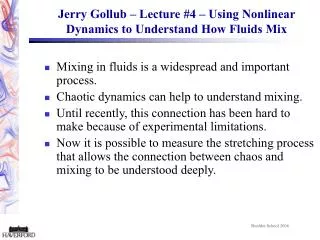
Jerry Gollub – Lecture #4 – Using Nonlinear Dynamics to Understand How Fluids Mix. Mixing in fluids is a widespread and important process. Chaotic dynamics can help to understand mixing. Until recently, this connection has been hard to make because of experimental limitations.

E N D
Jerry Gollub – Lecture #4 – Using Nonlinear Dynamics to Understand How Fluids Mix • Mixing in fluids is a widespread and important process. • Chaotic dynamics can help to understand mixing. • Until recently, this connection has been hard to make because of experimental limitations. • Now it is possible to measure the stretching process that allows the connection between chaos and mixing to be understood deeply.
Collaborators Greg Voth, now at Wesleyan Paulo Arratia, postdoc Greg Dobler and Tim Saint, undergraduates George Haller, MIT Earlier: L. Montagnon, E. Henry, D. Rothstein, W. Losert. NSF – DMR Haverford College
Types of Fluid Mixing • Turbulent mixing: Random structures produced by fluid instability at high Reynolds number Re stretch and fold fluid elements. • Chaotic mixing: Some laminar flows at modest Re can produce complex distributions of material. • Fundamental process (for both): repeated stretching and folding of fluid elements, which causes nearby points to separate from each other irreversibly.
2D Magnetically Driven Fluid Layer – (same for mixing and reaction studies) Glycerol and water a few mm thick, containing fluorescent dye. Electrodes Magnet Array Periodic forcing: Top View:
Mixing of a Dye Evolution of dye concentration field Same data updated once per period.
Precise Particle Tracking • ~ 800 fluorescent particles tracked simultaneously. • Positions are found to 40mm accuracy. • ~15,000 images: 40-80 images per period of forcing, and 240 periods. • Phase Averaging: 800*240 = 105 particles tracked at each phase.
Outline • Measuring velocity fields (time-periodic) • Mappings • Fixed points of the mappings • Hamiltonian chaos • Stretching fields • Using stretching to understand mixing • Extending the work: viscoelastic fluids • Using stretching to predict reaction progress • Teaching about fluids and nonlinear dynamics
Velocity Fields 0.9 cm/sec 0 (p=5, Re=56)
Why Do Periodic Flows Mix? Breaking Time Reversal Symmetry • To mix, the flow can be time periodic, but must not be time reversible: relative to any starting time. • Finite Reynolds numberRe=VL/n can break time reversal symmetry: Velocity at equal intervals before and after the moment of minimum velocity.
Particle Displacement Map: Unmixed Islands (Re=20, p=0.7) Line segments connect positions of particles one period apart; color indicated mag. of displacement
Particle Displacement Map at Higher Re • Lines connect position of each measured particle with its position one period later: Poincaré Map. No obvious connection to the vortices in the fluid. 0 cm 1.7 cm
Manifolds of Hyperbolic Fixed Points Unstable Manifold Stable Manifold Typical of Hamiltonian Chaos
Hamiltonian Chaos • Henri Poincaré first identified hyperbolic fixed points and their manifolds in the 3 body problem. • Structures like these are seen in many problems of Hamiltonian (conservative) chaos, e.g. forced oscillators; saturn’s rings, etc. Henri Poincaré (1854-1912) (from Barrow-Green, Poincaré and the three body problem, AMS 1997)
Why does mixing look like Hamiltonian chaos? Fluid Mixing Hamiltonian System Real Space Phase Space GeneralizedMomentum, p y x Generalized Position, q Stream Function Equations: Hamilton’s Equations: (Aref, J. Fluid Mech, 1984)
Pendulum Phase Plane – a simple hamiltonian system showing elliptic and hyperbolic points
Manifolds and Stretching Fields • The stable and unstable manifolds of hyperbolic fixed points form the building blocks of chaos. • These manifolds have been hard to extract from experiments. • Recent theoretical work has shown how to determine finite time stable and unstable manifolds using measurements of stretching in the flow. (Haller, Chaos 2000) • ... How can we measure stretching?
Definition of Stretching Stretching = lim (L/L0) L L0 0 Past Stretching Field: Stretching that a fluid element has experienced during the last Dt. (Large near unstable man.) Future Stretching Field: Stretching that a fluid element will experience in the next Dt. (Large near stable man.) L0
Past Stretching Field • Stretching is organized in sharp lines. Re=45, p=1, Dt=3
Future and Past Stretching Fields • Future Stretching Field (Blue) marks the stable manifold • Past Stretching Field (Red) marks the unstable manifold.
Future and Past Stretching Fields • Future Stretching Field (Blue) marks the stable manifold. • Past Stretching Field (Red) marks the unstable manifold. • Circles mark hyperbolic points. A “heteroclinic tangle”.
Stretching is Inhomogeneous: PDF Log(stretching) (Finite Time Lyap. Exp.) Stretching over one period Probability l / < l > Solid: Re=45, p=1, <l>=1.9 per-1 Dotted: Re=100, p=5, <l>=6.4 per-1 (Re=100,p=5)
Unstable manifold (past stretching field) and the dye concentration field • Lines of large past stretching (unstable manifold) are aligned with the contours of the concentration field. • This is true at every time (phase).
Homogenization: Decay of the Dye Concentration Field p=2, Re=65 110 periods
Decay of the Dye Concentration Field Log Contrast
Stretching - Summary • Particle tracking Velocity fields flow maps time-resolved stretching fields. • Ridges (lines) in the stretching field are unstable manifolds of hyperbolic “fixed” points in the flow. • The dye field contours align with the lines of maximal compression; lines of maximal stretching are along the concentration gradient. • Stretching PDF covers many decades; Mixing is highly inhomogeneous.
Non-Newtonian Fluids: Polymer solutions • Images of the dye field show changes in flow patterns and enhancement of mixing with a shear-thinning fluid. Shear-Thinning, Viscoelastic Newtonian • Newtonian, Re=1.25 • Shear-thinning, PAA 3000, Re=1.45, El=0.75, Cr =5.1 • Each row shows an image taken 10 periods after the one above it. Time
Shear-thinning breaks time-reversibility • Measure of the breaking of time reversal symmetry of periodic flows • Shear-thinning effects break time-reversibility
Application to Chemistry • Fast reactions are enormously enhanced by mixing. • Limited by diffusion into reaction zones, which is augmented by stretching. • The interplay between stretching, reaction, and diffusion has been studied numerically but not experimentally. • We measure stretching properties and use them to predict reaction progress. • P.E. Arratia and JPG; Supported by NSF-DMR - 0405187
Top View Electrodes Acid/Gly/H2O, Dye Gly/H2O, Salt Base/Gly/H2O A B Acid (HCl) + Fluorescein Base (NaOH) 12 cm Magnet Array 12 cm Magnets Experimental Set-up • Magnet spacing (L)= 2 cm • Typical frequency = 100 mHz • Sinusoidal Forcing • Particle diameter = 120 mm • CCD (1156x1024) @ 4 Hz
Fluorescence allows product concentration field to be measured H3O+ + OH- 2H2O A + B 2P • Pixel intensity is related to pH using a calibration curve. • We obtain the acid A(x,y,t) from the definition of pH • Product concentration is We also apply it locally (an approximation) We fit a logistic equation to the calibration curve.
Stretching=(dt+Dt)/ dt) Dt dt dt+Dt Stretching Fields • Measures the rate of divergence of nearby fluid elements; controls mixing efficiency.1 • Related to the local finite-time Lyapunov exponent • Measuring stretching fields: Particle tracks high spatial resolution velocity fields flow maps of particle displacements tt+Dt. • Stretching2 is computed from gradients of the flow maps. 1- Voth, G.A., et al., Phys. Fluids, 2003 2- G. Voth, G. Haller, & J.P. Gollub, Phys. Rev. Lett., 2002
(a) (b) (c) (d) Streamlines, and stretching fields (over 1 per.) Streamlines Stretching fields
Scaled Prob. Dist. of log Stretching after N periods(J. Stat. Phys. 2005) Log S scaled by the geometric mean stretching over the interval
Dynamics: A Basic Model A B - In a fast reaction the product forms at the boundary separating the reactants The reaction interface is stretched and folded by the chaotic flow At each point of the interface the flow can be decomposed into a convergent and a stretching direction
A Basic Model – (cont.) • The reaction is confined to the interface between acid and base. If the interface stretches at constant rate, its transverse thickness (after a short transient) is controlled by a balance between stretching and diffusion. • The product should grow exponentially at first, in proportion to the interface length, and then saturate when the interfaces become sufficiently close together.
1-100 periods Reactive Mixing: Product formation in time-periodic flows, Re=56 (p=2.5) Product Concentration is color-coded Random Array Regular Array Acid (HCl) + Fluorescein Base (NaOH) Acid (HCl) + Fluorescein Base (NaOH)
Effects of Order/Disorder and Re Re=37 Re=56 Re=56
Models • Exponential approach to saturation (dashed line) • Enhanced saturation – faster at late times (solid line) • The second model gives a good fit; possibly due to transportof reactants to pristine regions where they can react.
SUMMARY • Early product growth departs strongly from exponential behavior; we think it is due to the wide distribution of stretching rates. • Reaction progress is affected by spatial symmetry, and by the extent of departure from time-reversibility of the flow (determined by Re, etc.). • Normalized reaction product is well predicted for many flows by a single master curve depending on (mean Lyapunov exponent)(time), allowing prediction of the product simply by measuring stretching statistics.
Papers on mixing • G.A. Voth, G.H. Haller, and J.P. Gollub, "Experimental Measurements of Stretching Fields in Fluid Mixing", Physical Review Letters 88, 254501 (2002). • G.A. Voth, T. Saint, G. Dobler, and J.P. Gollub, “Mixing Rates and Symmetry Breaking in 2D Chaotic Flow”, Physics of Fluids 15, 2560-66 (2003). • P.E. Arratia and J.P. Gollub, “Mixing in Polymer Solutions: Effects of Shear Thinning”, Physics of Fluids 17, 053102 (2005). • P.E. Arratia and J.P. Gollub, “Predicting the Progress of Diffusively Limited Chemical Reactions in the Presence of Chaotic Advection”, Physical Review Letters 96, 024501 (2006).
Conclusion • Ideas from nonlinear dynamics contribute to understanding fluid phenomena. • Equally, fluids illuminate nonlinear dynamics and can be used to teach it. • Fluids ought to play a larger role in physics teaching. I make a case for this in Physics Today, December 2003: “One of the oddities of contemporary physics education is the nearly complete absence of continuum mechanics…” • More: www.haverford.edu/physics-astro/Gollub
Why not teach about continuum mechanics? • Widely used in astrophysics and biophysics. • Many applications to geophysical phenomena, soft condensed matter, complex fluids, etc. • But curricula are crowded, good texts are rare, and many of us feel unprepared. • Still, we can find space within various existing courses if we try. • A modern fluid mechanics course can showcase the diversity of physics and its connections.
Possible Benefits • Developing competence in using partial differential equations. • Introducing nonlinear dynamics: instabilities, chaotic dynamics, and complexity. • Motivating students by making connections to topics such as atmospheric dynamics, biological materials, astrophysics, etc. • Courses for non-majors: “Fluids in Nature”
How we do it: measuring stretching Flow Map is defined as: Right Cauchy-Green Strain Tensor • Stretching during time Dt is given by the square root of largest eigenvalue of Cij • This is a function of position, initial time, and time difference. • Stretching fields can be measured from either measured trajectories or integration of hypothetical particle motion in measured velocity fields.