Download

1 / 19
210 likes | 819 Views
Face Recognition Using Embedded Hidden Markov Model. Overview. Introduction. Motivation behind this research project. Markov Chains -- how to estimate probabilities. What is Hidden Markov Model (HMM). Embedded HMM. Observation Vectors. Training of face models. Face Recognition.

E N D
Overview • Introduction. • Motivation behind this research project. • Markov Chains -- how to estimate probabilities. • What is Hidden Markov Model (HMM). • Embedded HMM. • Observation Vectors. • Training of face models. • Face Recognition. • Conclusion.
Introduction • We implemented a real-time face recognition scheme “Embedded HMM” and compared it with the Human Visual System. • Embedded HMM approach uses an efficient set of observation vectors and states in the Markov chain.
Motivation • None of the researchers have compared how an objective measurement algorithm results (face recognition algorithm) perform against a subjective measurement (Human visual system). • Learning the inner details of face recognition algorithm, how it works and what it actually does to compare two faces, what are the complexities involved and what are the improvements possible in future.
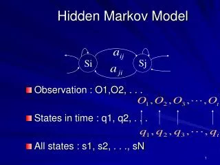
Markov Chains -- How to estimate probabilities • S is a set of states. Random process {Xt|t=1,2….} is a Markov Chain if t, the random variable Xt satisfies the Markov property. pij=P{Xt+1=j | Xt=i, Xt-1=it-1, Xt-2=it-2,…….X1=i1} = P{Xt+1=j | Xt=i } So, we have : P(X1X2…….Xk-1Xk)=P(Xk | X1X2……. Xk-1).P(X1X2…….Xk-1) =P(Xk | Xk-1).P(X1X2…….Xk-1) =P(X1). P(Xi+1 | Xi) for i=1,k-1 pij is called the transition matrix. Markov Model=Markov Chain + Transition matrix.
Hidden Markov Model • HMM is a Markov chain with finite number of unobservable states. These states has a probability distribution associated with the set of observation vectors. • Things necessary to characterize HMM are: -State transition probability matrix. -Initial state probability distribution. -Probability density function associated with observations for each of state.
Example Illustration N=number of states in model M=number of distinct observation symbols. T=length of a observation sequence (no of symbols) Observation symbols=(v1,v2,...vM). i=probability of being in state i at time 1(start). A={aij}=probability of state j at time t+1, given state i at time t. B={bjk}=prob of observing symbol vk in state j. Ot=observation symbol at time t. =(A,B, ) denotes the HMM model.
Cont… • O=O1…..OT is called the observation seq. • How did we get this ??? • How do we get the probability of occurrence of this sequence in the state model?? P(O| ) Hint: sum ( P(O| I,).P(I| )), where I=state sequence. • Find I such that we get Max P(O,I| ). (viterbi algorithm). • How do we find this I ??? Hint: Converts into minimization of path weight problem in graph.
HMM Model Face recognition using HMM
Cont… • How do we train this HMM?? Hint: Encode the given observation sequences in such a way that if a observation sequence having many characteristic similar to the given one is encountered later, it should identify it. (use k-means clustering algorithm)
K-means clustering explained… • Form N clusters initially. • Calculate initial probabilities and transition probabilities. (,A) • Find mean and covariance matrix for each state. • symbol probability distribution for each training vector in each state. (Gaussian Mixer). (B) • So =(A,B, ) as calculated above. • Find optimal I for each training sequence using this . • Re-assign symbols to different clusters if needed. • Re-calculate (HMM). Repeat until no re-assignments are possible.
Embedded HMM • Making each state in a 1-D HMM an HMM, makes an embedded HMM model with super states along with embedded states. • Super states model the data in one direction(top-bottom). • Embedded states model the data in another direction(left-right). • Transition from one super state to another is not possible. Hence named “Embedded HMM”.
Elements of Embedded HMM: • Number of super state: N0, set of super states: S0={S0,i} • Initial super state distribution, 0=(0,i), where 0,i are the • probabilities of being in super state i at time 0. • super state transition probability matrix: • A0={a0,ij}, where a0,ij is the probability of transitioning from • super state j to super state i. • Parameters of embedded HMM: • -Number of embedded states in the kth super state, • N1(k), and the set of embedded states S1(k)={S1,i(k)}. • -1(k)=(1,I(k)), where 1,I(k) are probabilities of being in state I of super state k at time 0. • -State transition probability matrix A1(k)={a1,ij(k)}
Cont.. • The state probability matrix B(k)={bi(k)(Ot0,t1)}, for set of observation vector at row t0, column t1. • Let (k)={1(k), A1(k), B(k)} is the set of parameter for kth super state. • So, Embedded HMM could be defined as: ={0 , A0 , }, where ={(1), (2),… (N0)}
Observation Vectors • P x L window scans the image from left-right and top-bottom, with overlap between adj windows is M lines vertically and Q columns horizontally. • Size of observation vectors = P x L. • Pixel value don’t represent robust features due to noise and changes in illuminations. • 2D-DCT coefficients in each image block.(low freq components, often only 6 coefficients). • This helps reduce size of obs_vector drastically.
Face recognition • Get the observation sequence of test image. (obs_test) • Given (1,…… 40) • Find likely hood of obs_test with each i. • The best likely hood identifies the person. • Likely Hood = P(obs_test| i) Hint:use viterbi algorithm again to get the sequence state for this obs_test sequence.
Conclusion • Small observation vector set. • Reduced number of transitions among states. • Lesser computing. • 98% real-time recognition rate. • Little overhead of complexity of algorithm.