Amortized Analysis

Amortized Analysis

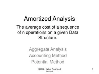
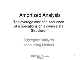
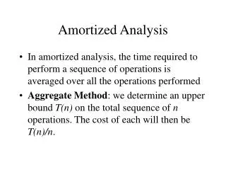
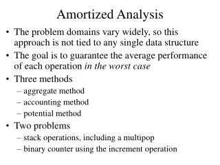
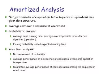
Amortized analysis: • Guarantees the avg. performance of each operation in the worst case. • Aggregate method • Accounting method • Potential method • Aggregate method • A sequence of n operations takes worst-case time T(n) in total. In the worst case, the amortized cost (average cost) per operation is T(n)/n

Eg.1 [Stack operation] PUSH(S,x): pushes object x onto stack S POP(S): pops the top of stack S and return the popped object Each runs in O(1) time (假設只需一單位時間) 故 n 個 PUSH 和 POP operations 需 (n) time 考慮MULTIPOP(S, k): pops the top k objects of stack S MULTIPOP(S, k) While not STACK-EMPTY(S) and k0 do { POP(S) k  k-1 } 故執行一 MULTIPOP 需 min{s, k} 個步驟

問題: 執行上述 PUSH, POP, MULTIPOP n次 假設 initial stack 為 empty 試問每一 operation 在 worst-case 之 amortized cost? • Each object can be popped at most once for each time it is pushed. • 上述問題只需 O(n) time O(n)/n = O(1) 每個 operation 平均所需的時間

Eg.2 [Incrementing a binary counter] A k-bit binary counter, counts upward from 0 A[k-1] A[k-2]…A[1] A[0] highest order bit lowest order bit Increment(A) { i  0; while i<length[A] and A[i]=1 do A[i]  0; i  i+1; if i<length[A] then A[i]  1; } Ripple-carry counter A[7]A[6]A[5]A[4]A[3]A[2]A[1]A[0] 0 0 0 0 0 0 0 0 0 0 0 0 0 0 0 1 0 0 0 0 0 0 10 0 0 0 0 0 0 1 1 0 0 0 0 0 100 0 0 0 0 0 1 0 1 0 0 0 0 0 1 10 0 0 0 0 0 1 1 1 0 0 0 0 1000 0 0 0 0 1 0 0 1 0 0 0 0 1 0 10 0 0 0 0 1 0 1 1 0 0 0 0 1 1 00

問題: 執行 n 次(依序) Increment operations. 在 worst-case 每一operation 之 amortized cost 為何? • A[0] 每 1 次改變一次 A[1] 每 2 次改變一次 A[i] 每 2i次改變一次故 amortized cost of each operation 為 O(n)/n = O(1)

Accounting method: • Assign differing charges to different operations close to actual charge (amortized cost) If the amortized cost > actual cost, the difference is treated as credit (在aggregate method所有operation有相同的amortized cost) • 選擇(定義)每一operation之適當 amortized cost 需注意: 1. 若要每一 op 在 worst-case 之平均 cost小, 則一串 operations 之 total amortized cost必須  total actual cost 2. Total credit 必須是非負

Eg. 1 [Stack operation] Amortized cost: PUSH 2 , POP 0 , MULTIPOP 0 Actual cost: PUSH 1 , POP 1 , MULTIPOP min(k,S) 在 PUSH 之 amortized cost 中預支了 POP 時所需之 cost 故在 n 個運作之後, total amortized cost = O(n) • Eg. 2 [Increment a binary counter] Set a bit to 1: amortized cost 2 Reset a bit to 0: amortized cost 0 在 Increment procedure 中每次最多只 set 一個 bit 為 1 故每次最多 charge 2, 執行 n 次 Increment 其 total amortized cost = O(n)

Potential method • D0 : initial data structure ci : actual cost of the i-th operation Di : data structure after applying the i-th operation to Di-1  : potential function (Di) is a real number : the amortized cost of the i-th operation w.r.t potential function is 若 (Dn)  (D0), 則 total amortized cost 為 total actual cost 之一 upper bound

Eg. 1 [Stack operation] 定義 potential function : stack size (D0)=0, 亦知 (Di)  0 i-th op. PUSH: MULTIPOP(S, k): 令 k’=min{k,S} POP: 同理所以一序列 n 個 op 之 total amortized cost 為 O(n)

Eg. 2 [Incrementing a binary counter] 對 counter 而言其 potential function 值為在 i-th op 後被設定為 1 的 bit 個數 bi = # of 1’s in the counter after the i-th operation • Suppose that the i-th Increment op. resets ti bits Actual cost  ti+1 • # of 1’s in the counter after the i-th op.: bi  bi-1 –ti + 1

front rear Stack A Stack B • Implement a Queue with two Stacks: Stack A : Dequeue Stack B : Enqueue SB : stack size of B • Enqueue(x) { PUSH(B, x) } Dequeue(Q) { if Empty(Q) then return “empty queue”; else if Empty(A) then while not Empty(B) do PUSH(A, POP(B); POP(A); }

(Di)=2[stack size of B after the i-th operation] Enqueue: Dequeue:

Dynamic tables: Operations:Table-Delete, Table-Insert Load factor: = (number of items)/(table size) Define the load factor of an empty Table as 1. TableT:

Table expansion: Table-Insert(T, x) { if size[T]=0 then allocate table[T] with 1 slot size[T]=1; if num[T]=size[T] then {allocate new-table with 2*size[T] slots;  Expansion insert all items in table[T] into new-table; free table[T]; table[T] = new-table; size[T] = 2*size[T];} insert x into table[T]; num[T]= num[T] + 1;}

Define potential function No expansion after the ith op: With expansion after the ith op:

Table expansion and contraction: I, D, I, I, D, D, I, I, I………. : A sequence of n operations. Preserve two properties: . Load factor is bounded below by a constant. . The amortized cost of a table op is bounded above by a const. Strategy: .Double the table size when an item is inserted into a full table. .Halve the table size when a deletion causes the table to become less than ¼ full.

Define potential function: If the i-th operation is Table-Insert: If the load factor >= ½, then the analysis is the same as before.

If the i-th operation is Table-Delete:

Exercise! 17.4-2.

Amortized Analysis