Download
1 / 18
180 likes | 313 Views
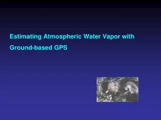
Estimating Atmospheric Water Vapor with Ground-based GPS Lecture 12. Overview. This lecture covers metrological applications of GPS Some of the material has already been presented and is shown here for completeness. There are two major contributions of the atmosphere:

E N D
Estimating Atmospheric Water Vapor with Ground-based GPSLecture 12
Overview • This lecture covers metrological applications of GPS • Some of the material has already been presented and is shown here for completeness. • There are two major contributions of the atmosphere: • Neutral atmospheric delay composed of hydrostatic component (N2, O2, CO2, trace gases and part of the water vapor contribution) and water vapor component • Ionospheric delay component due to free electrons. This component is frequency dependent and can be estimated from dual frequency measurements (L1 and L2 frequencies) MetApps Lec 12
Atmospheric Delays Ionosphere (use dual frequency receivers) Troposphere (estimate troposphere) Ionosphere Troposphere MetApps Lec 12
Sensing the Atmosphere with Ground-based GPS The signal from each GPS satellite is delayed by an amount dependent on the pressure and humidity and its elevation above the horizon. We invert the measurements to estimate the average delay at the zenith (green bar). ( Figure courtesy of COSMIC Program )
Multipath and Water Vapor Effects in the Observations One-way (undifferenced) LC phase residuals projected onto the sky in 4-hr snapshots. Spatially repeatable noise is multipath; time-varying noise is water vapor. Red is satellite track. Yellow and green positive and negative residuals purely for visual effect. Red bar is scale (10 mm). MetApps Lec 12
Sensing the Atmosphere with Ground-based GPS Colors are for different satellites Total delay is ~2.5 meters Variability mostly caused by wet component. Wet delay is ~0.2 meters Obtained by subtracting the hydrostatic (dry) delay. Hydrostatic delay is ~2.2 meters; little variability between satellites or over time; well calibrated by surface pressure. Plot courtesy of J. Braun, UCAR MetApps Lec 12
Effect of the Neutral Atmosphere on GPS Measurements Slant delay = (Zenith Hydrostatic Delay) * (“Dry” Mapping Function) + (Zenith Wet Delay) * (Wet Mapping Function) + (Gradient Delay NS) ( Gradient Mapping Function) * Cos/Sin(Azimuth) • To recover the water vapor (ZWD) for meteorological studies, you must have a very accurate measure of the hydrostatic delay (ZHD) from a barometer at the site. • For height studies, a less accurate model for the ZHD is acceptable, but still important because the wet and dry mapping functions are different (see next slides) • The mapping functions used can also be important for low elevation angles • For both a priori ZHD and mapping functions, you have a choice in GAMIT of using values computed at 6-hr intervals from numerical weather models (VMF1 grids) or an analytical fit to 20-years of VMF1 values, GPT and GMF (defaults) MetApps Lec 12
Mapping function effects • Mapping functions differ and this means hydrostatic and wet delays are coupled in the estimation. • Example: Percent difference (red) between hydrostatic and wet mapping functions for a high latitude (dav1) and mid-latitude site (nlib). Blue shows percentage of observations at each elevation angle. From Tregoning and Herring [2006]. MetApps Lec 12
Effect of surface pressure errors a) surface pressure derived from “standard” sea level pressure and the mean surface pressure derived from the GPT model. b) station heights using the two sources of a priori pressure.c) Relation between a priori pressure differences and height differences. Elevation-dependent weighting was used in the GPS analysis with a minimum elevation angle of 7 deg. MetApps Lec 12
Short-period Variations in Surface Pressure not Modeled by GPT • Differences in GPS estimates of ZTD at Algonquin, NyAlessund, Wettzell and Westford computed using static or observed surface pressure to derive the a priori. Height differences will be about twice as large. (Elevation-dependent weighting used). MetApps Lec 12
Example of GPS Water Vapor Time Series GOES IR satellite image of central US on left with location of GPS station shown as red star. Time series of temperature, dew point, wind speed, and accumulated rain shown in top right. GPS PW is shown in bottom right. Increase in PW of more than 20mm due to convective system shown in satellite image. MetApps Lec 12
Water Vapor as a Proxy for Pressure in Storm Prediction Correlation (75%) between GPS-measured precipitable water and drop in surface pressure for stations within 200 km of landfall. GPS stations (blue) and locations of hurricane landfalls J.Braun, UCAR MetApps Lec 12
GAMIT Meteorological Apps. • For gamit meteorological applications the zenith delays and gradient estimates are of most interest. • In general, we find at least two gradient parameters per day (i.e., a linear change over 24-hrs) should be used for good station coordinate estimates. • For atmospheric delay estimates, one strategy is to tightly constrains coordinates in gamit (based on very good coordinates). One potential problem here, is loading effects can change the coordinates and thus possible alias into atmospheric delay estimates. • The sh_metutil is a script that will generate water estimates from gamit o-files is there is a source of pressure data (gamit z-file or rinex met file). MetApps Lec 12
Ionospheric delay estimates • GAMIT uses a dual frequency combination to eliminate the ionospheric delay (to first order) from the data observable. • There are no utilities in gamit to estimate ionospheric delay robustly. • The one-way phase residual files from autcln could be used but the pseudoranges in gamit are not corrected for P1-P2 biases (because these cancel out in double differences). The C1-P1 bias (differential code biases) are accounted for provide dcb.dat is up to date. • http://aiuws.unibe.ch/ionosphere/p1p2_all.dcb provides P1-P2 bias estimates and these need to be applied to one-way range residuals to obtain resonable estimates of the absolute ionospheric delays. MetApps Lec 12
Influence of the Atmosphere Atmospheric and Ionospheric Effects Precipitable Water Vapor (PWV) derived from GPS signal delays Assimilation of PW into weather models improves forecasting for storm intensity Total electron count (TEC) in Ionosphere MetApps Lec 12 16
Suominet – PBO Stations • 80 Plate Boundary Observatory (PBO) sites now included in analysis. • These sites significantly improve moisture observations in western US. • Should be useful for spring/summer precipitation studies. • Network routine exceeds 300 stations. MetApps Lec 12
Impact of GPS PW on Hurricane Intensity Dean - 2007 Gustav - 2008 MetApps Lec 12