Download
1 / 22
220 likes | 269 Views
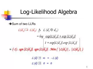
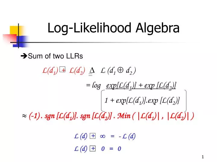
= - L (d). L (d). +. L (d). 0 = 0. +. Log-Likelihood Algebra. Sum of two LLRs L(d 1 ) + L(d 2 ) L ( d 1 d 2 ) = log exp[L(d 1 )] + exp [L(d 2 )] 1 + exp[L(d 1 )].exp [L(d 2 )]

E N D
= - L (d) L (d) + L (d) 0 = 0 + Log-Likelihood Algebra Sum of two LLRs L(d1) + L(d2) L (d1 d2 ) = log exp[L(d1)] + exp [L(d2)] 1 + exp[L(d1)].exp [L(d2)] (-1) . sgn [L(d1)]. sgn [L(d2)] . Min ( |L(d1)| , |L(d2)| )
Iterative decoding example • 2D single parity code • di di= pij
Iterative decoding example • Estimate Lc(xk) • = 2 xk /2 • assuming 2= 1
Leh( d1) = [Lc ( x 2) + L(d2) ] Lc ( x 12 ) = new L( d1 ) Leh( d2) = [Lc ( x 1) + L(d1) ] Lc ( x 12 ) = new L(d2) Leh( d3) = [Lc ( x 4) + L(d4) ] Lc ( x 34 ) = new L(d3) Leh( d4) = [Lc ( x 3) + L(d3) ] Lc ( x 34 ) = new L(d4) + + + + Iterative decoding example • Compute • Le( dj ) = [Lc ( x j) + L(dj ) ] Lc ( x ij) +
Lev( d1) = [Lc ( x 3) + L(d3) ] Lc ( x 13 ) = new L( d1 ) Lev( d2) = [Lc ( x 4) + L(d4) ] Lc ( x 24 ) = new L(d2) Lev( d3) = [Lc ( x 1) + L(d1) ] Lc ( x 13 ) = new L(d3) Lev( d4) = [Lc ( x 2) + L(d2) ] Lc ( x 24 ) = new L(d4) + + + + ^ ^ ^ L( di ) = Lc ( x i) + Leh(di) + Lev( dj ) Iterative decoding example After many iterations the LLR is computed for decision making
Parallel Concatenation Codes • Component codes are Convolutional codes • Recursive Systematic Codes • Should have maximum effective free distance • Large Eb/No maximizing minimum weight codewords • Small Eb/No optimizing weight distribution of the codewords • Interleaving to avoid low weight codewords
{uk} + L-1 L-1 uk = g1i dk-i (mod 2) ; i=1 vk = g2i dk-i (mod 2) ; i=1 {dk} dk-1 dk-2 dk + {vk} Non - Systematic Codes - NSC G1 = [ 1 1 1 ] G2 = [ 1 0 1 ]
{dk} {uk} ak-1 ak-2 ak + + {vk} L-1 ak = dk + gi’ ak-i (mod 2) ; gi’ = g1i if uk = dk i=1 g2i if vk = dk Recursive Systematic Codes - RSC
NSC RSC Trellis for NSC & RSC 00 00 a = 00 a = 00 11 11 11 11 b = 01 b = 01 00 00 10 10 c = 10 c = 10 01 01 01 01 d = 11 d = 11 10 10
+ + ak-1 ak-1 ak-2 ak-2 ak ak + + {v2k} {v1k} Concatenation of RSC Codes {dk} {uk} Interleaver {vk} { 0 0 …. 0 1 1 1 0 0 …..0 0 } { 0 0 …. 0 0 1 0 0 1 0 … 0 0 } produce low weight codewords in component coders
APP Joint Probability ki,m = P { dk = i, Sk = m / R1 N } State at time k Received sequence From time 1 to N APP P { dk = i / R1 N } = ki,m ; i = 0,1 for binary m k0,m k1,m k0,m k1,m m m m m Likelihood Ratio ( dk ) = Log Likelihood Ratio L( dk ) = Log Feedback Decoder
Feedback Decoder • MAP Rule dk =1 ; L(dk) > 0 dk =0 ; L(dk) < 0 ^ ^ L( dk) = Lc ( x k) + L(dk) + Le( dk ) L1( dk ) = [Lc ( x k) + Le1(dk ) ] L2( dk ) = [ f{L1 ( dn) }n k + Le2(dk ) ]
Le2( dk ) L2( dk ) xk L1( dn ) L1( dk ) De-Interleaver DECODER 1 DECODER 2 De-Interleaver Interleaver y1k y2k yk dk Feedback Decoder
Modified MAP Vs. SOVA • SOVA • Viterbi Algorithm acting on soft inputs over forward path of the trellis for a block of bits • Add BM to SM compare select ML path • Modified MAP • Viterbi Algorithm acting on soft inputs over forward and reverse paths of the trellis for a block of bits • Multiply BM & SM Sum in both directions best overall statistic
{uk} dk-1 dk-2 dk {dk} + {vk} MAP Decoding Example 00 a = 00 11 b = 10 00 11 01 c = 01 10 01 d = 11 10
Branch Metric ki,m = P { dk = i, Sk = m , Rk } = P { Rk / dk = i, Sk = m } . P {Sk = m / dk = i } . P { dk = i } ki,m = P { xk / dk = i, Sk = m } . P { yk / dk = i, Sk = m } . { ki / 2L } P {Sk = m / dk = i } = 1 / 2 L = ¼ ; P { dk = i } = 1 / 2 ; MAP Decoding Example • d = { 1, 0, 0 } • u = { 1, 0, 0 } x = { 1., 0.5, -0.6 } • v = { 1, 0, 1 } y = { 0.8, 0.2, 1.2 } • Apriori probabilities 1 = 0 = 0.5
ki,m = ki,m = Assuming Ak = 1 2 =1 ; ki,m = 0.5 exp { xk . uki + yk . vki,m } { ki / 2L } (1/2 ) exp { - (xk – uki )2 /(2 2 ) }dxk { Ak ki } exp { (xk . uki )+ (yk . Vki,m )/ 2 } ki,m = P { xk / dk = i, Sk = m } . P { yk / dk = i, Sk = m } . { ki / 2L } MAP Decoding Example For AWGN channel : . (1/2 ) exp { - (yk – vki,m )2 /(2 2 ) }dyk
ki,m = 0.5 exp { xk . uki + yk . vki,m } 1 k+1m= ki,b(j,m) kb(j,m) J=0 Subsequent steps • Calculate branch metric • Calculate forward state metric • Calculate reverse state metric 1 km= kj,m k+1f(j,m) J=0
km k1,m k+1f(1,m) km k0,m k+1f(0,m) m m Subsequent steps • Calculate LLR for all times Log Likelihood Ratio L( dk ) = Log • Hard decision based on LLR
{ k1} km exp { xk . uk1 + yk . Vk1,m } k+1f(1,m) m { k0} km exp { xk . uk0 + yk . Vk0,m }k+1f(0,m) m km exp { yk . Vk1,m } k+1f(1,m) m { k} exp { 2xk } km exp { yk . Vk0,m }k+1f(0,m) m LLR L( dk ) = L(dk) + { 2xk } + Log [ke ] Iterative decoding steps Likelihood Ratio ( dk ) = = = { k} exp { 2xk } { k e}
ki,m = ke i exp { xk . uki + yk . Vki,m } km k1,m k+1f(1,m) km k0,m k+1f(0,m) m m Iterative decoding • For the second iteration; • Calculate LLR for all times Log Likelihood Ratio L( dk ) = Log • Hard decision based on LLR after multiple iterations