Download
1 / 45
450 likes | 566 Views
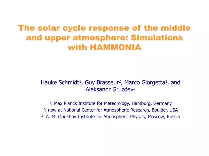
The solar cycle response of the middle and upper atmosphere: Simulations with HAMMONIA. Hauke Schmidt 1 , Guy Brasseur 2 , Marco Giorgetta 1 , and Aleksandr Gruzdev 3 1 : Max Planck Institute for Meteorology, Hamburg, Germany 2 : now at National Center for Atmospheric Research, Boulder, USA

E N D
The solar cycle response of the middle and upper atmosphere: Simulations with HAMMONIA Hauke Schmidt1, Guy Brasseur2, Marco Giorgetta1, and Aleksandr Gruzdev3 1: Max Planck Institute for Meteorology, Hamburg, Germany 2: now at National Center for Atmospheric Research, Boulder, USA 3: A. M. Obukhov Institute for Atmospheric Physics, Moscow, Russia
Outline • HAMMONIA - Model description • The atmospheric response to the 27-day variation • The atmospheric response to the 11-year solar cycle • Energy budget • Chemistry • Dynamics • The atmospheric response to CO2 doubling
~ 250 km Ion Drag Molecular Processes IR Cooling (non-LTE) Solar Heating (SRB&C, Ly-a, EUV) Chemical heating Gravity Wave Drag ~ 80 km HAMMONIA Solar Heating (near UV, vis. & near IR) Clouds & Convection Turbulent Diffusion ~ 30 km Surface Fluxes IR Cooling HAMMONIA – a member of the ECHAM family Neutral Gas Phase Chemistry (MOZART3) MAECHAM5 ECHAM5
HAMMONIA - Description (1) • 67 levels from the surface to ~250 km, T31 horizontal resolution • Based on ECHAM/MAECHAM5 with extensions to account for processes in the upper atmosphere • Radiation • Near UV, Vis. & near IR heating: 4 bins, Fouquart & Bonnel (Contr. Atm Phys., 1980); or taken from TUV (< 680nm) • IR cooling: RRTM from Mlawer et al. upto 0.1 hPa (eg. Iacono et al., JGR, 2000) • Non-LTE IR cooling: 15 μm CO2 & 9.6 μm O3 above 0.02 hPa (Fomichev, JGR, 1998) • CO2-IR heating (Ogibalov & Fomichev, Adv. Sp. Res., 2003) • EUV heating: 5 to 105 nm, 20 bins, Richards et al. (JGR, 1994), efficiency from Roble (AGU Monogr., 1995) • Schumann Runge B&C heating: either Strobel (JGR, 1978), eff. from Mlynczak & Solomon (JGR, 1993); or taken from TUV
HAMMONIA - Description (2) • Doppler-spread non-orographic gravity wave drag (Hines, JASTP, 1997) and orographic gravity wave drag (Lott, MWR, 1999) • Prescribed ion drag (Hong & Lindzen, JAS, 1996) • Molecular processes • Chemistry of the MOZART-3 CTM (48 constituents, 153 gas phase reactions) • Chemical lower boundary concentrations from MOZART-2 simulations • Photodissociation rate computation from MOZART-3 (based on TUV, Madronich et al.) • JO2: Chabrillat & Kockaerts (Lya, GRL, 1998), Brasseur & Solomon (SRC, Book, 1986), Koppers & Murtagh (SRB, Ann. Geoph., 1996) • JNO: Minschwaner & Siskind (JGR, 1993) • Chemical heating for 7 reactions • R and Cp height dependent
Acknowledgements • People at (or formerly at) MPI-Met: • M. Charron, T. Diehl, M. Giorgetta, E. Manzini, and E. Roeckner and the ECHAM-team • People who contributed to the model development outside MPI-Met: • V. Fomichev1, D. Kinnison2, and S. Walters2 • 1 York University, Toronto, Canada • 2 NCAR, Boulder, USA • J. Lean (Naval Res. Lab., Washington, USA) provided the solar irradiance spectra • D. Marsh (NCAR) helped in the model evaluation with SABER data • M. Zecha and P. Hoffmann (IAP Kühlungsborn) for model evaluation with ground-based observations • Computations were made at the DKRZ (German climate computing centre) • The work was supported by the BMBF (German ministry for education and science)
Zonal mean temperature [K], July, 16 LT HAMMONIA SABER/TIMED, July 1-16, 2002
Zonal mean O3 [ppmv], July, 15 LT SABER/TIMED, July 6-14, 2002 HAMMONIA URAP
Zonal mean zonal wind [m/s], July UARS (HRDI) / UKMO HAMMONIA
Temperature in the Mesopause RegionHAMMONIA – Meteor Radar Observations (courtesy by M. Zecha, IAP Kühlungsborn, Germany, for meteor radar details, see e.g. Singer et al., JASTP, 2004)
Variability of solar irradiance as given by UARS / SOLSTICE (Maximum: 1992, Minimum: 1996) (Rottmann, Space Sc. Rev., 2000)
Penetration depth of solar radiation in the atmosphere (Liou, Academic Press, 2002) 50 100 150 200 250 300 (nm)
normalized intensity normalized intensity The variation of solar UV radiation (Rottman, Sp. Sc. Rev., 2000) Fig. 5: The variation of the solar UV-radiation in the spectral range from 160 to 170 nm expressed as a normalized intensity observed by the SOLSTICE instrument. The figure shows a prominent short term (quasi 27-day) variability with strongly changing amplitude within the course of the 11-year solar cycle. (Figure taken from Rottman, Space Sc. Rev., 2000.)
27-day Variation Experiments - Setup Two simulations over 5 years each: • forced by mean solar irradiance as for January to June 1990 • as in a) but with an additional 27-day variation of solar irradiance • irradiance variation is assumed to be sinusoidal and have a period of exactly 27 days • irradiance depending on wavelength (1nm resolution, see Lean et al., JGR, 1997) for λ>120nm has been analysed spectrally for Jan-Jun 1990 • the analysed amplitude for the 27-day period was used as amplitude of our artificial forcing • EUV is modulated using F10.7 as proxy (Richards et al., JGR, 1994) • SSTs fixed to climatological values • compound concentrations at the surface are fixed to climatological values
no forcing The 27-day solar signal in low-latitude ozone
winter summer 250 250 2.0 1.5 1.5 1.0 200 200 0.5 1.0 0.0 0.5 -0.5 0.0 -1.0 -0.5 ) ) -1.5 150 150 -1.0 m m -2.0 k k ( ( -1.5 -2.5 t t h h -2.0 -3.0 g g i i -3.5 -2.5 e e 100 100 H H -4.0 -3.0 -4.5 -3.5 -5.0 -4.0 -5.5 -4.5 50 50 -6.0 -5.0 -6.5 0 0 10 20 30 40 50 10 20 30 40 50 Period (day) Period (day) The 27-day solar signal in mid-latitude ozone Normalized Ozone Power Spectra at 50N
Ozone running spectrum at 35 km at 50S 50 -11.0 -11.5 40 ) -12.0 y a -12.5 d ( 30 -13.0 d o i -13.5 r e -14.0 P 20 -14.5 -15.0 10 1.5 2.0 2.5 3.0 3.5 4.0 4.5 5.0 5.5 Year of simulation The 27-day solar signal in stratospheric ozone
Solar Cycle Experiments - Setup Two simulations over 20 years forced by constant solar irradiance for • solar minimum (September 1986, F10.7=69) • solar maximum (November 1989, F10.7=235) • irradiance depending on wavelength (1nm resolution) from Lean et al. (JGR, 1997) for λ>120nm • EUV is modulated using F10.7 as proxy (Richards et al., JGR, 1994) • upper boundary condition for H und O from MSISE90 is modulated using F10.7 as proxy (Hedin, JGR, 1992) • thermospheric solar NO production is increased by 1/3 for high activity • NO production by galactic cosmic rays is modulated • SSTs fixed to climatological values • Compound concentrations at the surface fixed to climatological values
Solar cycle effect on the global mean energy budget solar heating (incl. chemical) infrared cooling molecular diffusion solar minimum solar maximum
Solar cycle effect on the energy budget(annual mean, K/day) solar heating chemical heating long wave heating/cooling molecular diffusion (heat conduction)
Solar cycle effect - annual mean delta T [vmr], (solar max – min) delta T, significance delta O3 [%], (solar max – min) delta O3, significance
Solar cycle effect on temperaturesimulation vs. observations(observed values are adapted from papers listed by Beig et al., Rev. Geophys., 2003) delta T [K], annual zonal mean, (solar max – min) 0d 10d 3-10b 8d a: French, PhD thesis, 2002, OH b: Reisin & Scheer, Ph. Ch. Earth, 2002, OH, O2 c: Mohanakumar, Ann. Geo., 1995, rockets d: She & Krueger, Adv Sp. Res., 2003, lidar e: Lowe, workshop paper, 2002, OH f: Keckhut et al., JGR, 1995, lidar g: Semenov, Ph. Ch. Earth, 2000, OH h: Offerman et al., Adv. Space Res., 2003, OH j: Espy & Stegmann, Ph. Ch. Earth, 2002, OH k: Luebken, GRL, 2000, rockets m: Sigernes et al., JGR, 2003, OH #: zero or at least no significant trend 8a 0#,b 2e 8g 5h 3j 0#,m 0d -1f 0#,k 15c 4f
Height vs. Pressure in HAMMONIA solar min (1*CO2) solar max – solar min 2*CO2 – 1*CO2 dashed: negative values
Solar cycle effect - annual mean delta T [vmr], (solar max – min) delta T, significance delta O3 [%], (solar max – min) delta O3, significance
Solar cycle effect on annual mean stratospheric ozone(Lee and Smith, JGR, 2003) Satellite observations 2D-model results
delta O3 [%], July, (high - low) activity delta O3 [%], July, (high - low) activity O3 [vmr], July, low activity Solar cycle effect on July ozone Confidence level of delta O3 [%]
0 4 8 12 16 20 0 0 4 8 12 16 20 0 local time local time The solar cycle effect on the diurnal variation of ozone at the mesopause
Noctilucent Clouds(Polar Mesospheric Clouds) • Occur at the summer mesopause, depending on • Temperature (< 150 K) • Water vapor • Condensation nuclei
Solar Cycle and Polar Mesospheric Clouds (DeLand et al., JGR, 2003)
delta T [K], July, (high - low) activity delta T [K], July, (high - low) activity T [K], July, low activity Solar cycle effect on temperature Confidence level of delta T [%]
Solar cycle effect on wintertime zonal mean zonal wind (solar max-solar min) – Northern hemisphere NCEP analyses, (Kodera & Kuroda, JGR, 2002; Matthes et al., JGR, 2004) HAMMONIA
Solar cycle effect on wintertime zonal mean zonal wind (solar max-solar min) – Northern hemisphere NCEP analyses, (Matthes et al., JGR, 2004) old simulations, 10 years HAMMONIA
Solar cycle effect on wintertime zonal mean zonal wind (solar max-solar min) – Northern hemisphere (Shibata and Kuroda, JASTP, 2005)
MA-ECHAM5: The QBO simulated by MA-ECHAM5 (Giorgetta et al., GRL, 2002)
Solar cycle effect on temperature – the longitudinal dependence, January
CO2 doubling Experiments - Setup Four simulations over 10 years each 1) surface CO2 of 360 ppm (same run as „solar minimum“) 2) surface CO2 of 720 ppm + changed SST (and sea ice) • initial concentrations doubled to 720 ppm, followed by a one year initialization phase • sea surface temperatures and sea ice are taken from a respective run with a coupled ocean-atmosphere model (ECHAM5 + MPI-OM) 3) only SST changed (according to a CO2 concentration of 720 ppm) 4) only CO2 increased to 720 ppm
Effect of CO2 doubling and SST change on Temperature delta T, July CO2 + SST changed delta T, July only SST changed delta T, July only CO2 changed
Effect of CO2 doubling and SST change on Temperature delta T, July experiment where CO2 + SSTs are changed simultaneously delta T, July sum of two experiments where CO2 and SSTs are changed separately
Effect of CO2 doubling and SST change on July zonal wind u [m/s], July CO2 + SST changed only SST changed only CO2 changed delta u [m/s], July delta u [m/s], July delta u [m/s], July
Conclusions • The response to the 27-day variation is highly variable in space and time. • 11-year cycle effects in the MLT are strong. • The magnitude of the stratospheric ozone and temperature response is in agreement with observations. – How sure are we about the response in the real atmosphere? • The solar signal in stratospheric model winds is not robust. – How robust is the signal in the real atmosphere? • The solar signal depends on longitude and local time (tides!). • Changes of SSTs have an influence at least up to the mesopause.
The End Schmidt et al., The HAMMONIA chemistry climate model: Sensitivity of the mesopause region to the 11-year solar cycle and CO2 doubling, J. Climate, in press, 2006. available at http://www.mpimet.mpg.de/~schmidt.hauke/publications.php