Download
1 / 41
410 likes | 520 Views
Learning Probabilistic Environmental Models with Vision: Successes and Challenges. Our Interests and Perspective. Our interests: Not just SLAM, but modeling whole environment place recognition object classification e.g., grasping/manipulation Our perspective:

E N D
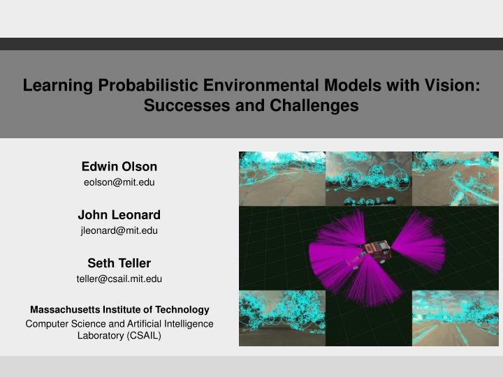
Learning Probabilistic Environmental Models with Vision: Successes and Challenges
Our Interests and Perspective • Our interests: • Not just SLAM, but modeling whole environment • place recognition • object classification • e.g., grasping/manipulation • Our perspective: • Long history of LIDAR-based SLAM • Vision-based • City Scanning • Omni-Bike • SIFT • DARPA Urban Challenge Edwin Olson
Why Vision? • Existence proof of successful vision-based systems • Passive • No interference • No safety hazard to humans • Cheap, low-power sensors • Human interoperability • Our world is designed for seeing animals • Promise of low-power processing • Not currently, though! • ~3 kW for Talos cameras • e.g., MERL Artificial Retina Edwin Olson
Non-vision state-of-the-art • Significant successes with laser, sonar, LBL data • Large environments • Fast and robust algorithms • Not quite a “solved” problem, but we’re getting there! • Perceptual Ambiguities • Optimization • Success correlated with sensor price… Edwin Olson
Vision state-of-the-art • Smaller environments • (Davison, Lowe, etc.) Elinas, Little. IROS 2007 Edwin Olson
Central Vision Challenges • Why is vision so much harder? • Data overload • Feature detectors designed via trial-and-error • Perceptual ambiguity • Bearing-only • DGC experience: • Computer vision is a man-hour black hole. Edwin Olson
Our work in vision navigation • Lane Detection • Feature-based methods • Lines + Points (omni-bike) • SIFT • Hypothesis filtering • Optimization instability Edwin Olson
Vision-based Lane Detection • One finalist team used vision-derived lane tracking • “Simple” vision problem • It’s hard Edwin Olson
Simplifying the problem • Reasonable prior • Mask non-lanes • LIDAR-based obstacles • Sun tracking Edwin Olson
Horizontal filter Road Paint Detector • Matched filter for road paint • Computationally affordable • Runs vertically and horizontally • Mask out self, obstacles, sky Edwin Olson
Road Paint Detector • Fit hermite splines to local maxima of filter response • RANSAC • Reject curves that point towards sun • GPS/IMU used to compute ephemeris • Used two similar implementations with different pro/cons! Edwin Olson
Lane Estimation • Accumulate lane center evidence in grid map • Lane boundary detections imply lane center 2m away • Bright = likely to be center of lane Edwin Olson
Lane Estimation Edwin Olson
Feature-based Methods • Interest points (e.g., Harris corners) • Relatively easy to extract • Each feature is fairly ambiguous • Data association is harder Edwin Olson
Omnibike (Mike Bosse’s PhD Work) Edwin Olson
Omnibike Results Edwin Olson
1.9km Vision Data Set • Monocular, w/odometry • MIT’s Talos • Five calibrated cameras, minimal overlap • High-end IMU+GPS for ground truth 1.9km path, three loops Degraded dead reckoning Edwin Olson
Scale Invariant Feature Transform (SIFT) • Matching features is error prone • Errors can lead to catastrophically bad models • SIFT Strategy: find the most recognizable features we can • 128 dimensional vectors • Hypotheses tend to be good (but not error free!) • Throws away huge amounts of information to achieve this Edwin Olson
SIFT Hypothesis Generation Edwin Olson
SIFT Landmark Initialization • SIFT observations provide vehicle-relative bearing only • Instantiate SIFT landmarks • Group SIFT detections • Initialize features via triangulation • Product: • Clouds of fully-localized SIFT features for each robot position Lowe 1999 Edwin Olson
SIFT Hypothesis Generation • When we revisit an area, • Try to match SIFT features seen at each time • Find consistent set of correspondences • Random sample consensus (RANSAC) • Fit rigid-body transformation to correspondences using Horn’s algorithm • Output: a new contraint between two poses Feature correspondences allow a hypothesis to be computed t = 174 s t = 31 s Fischler & Bolles, 1981 Edwin Olson
d=128 Posterior pose graph, SIFT d = 128 time Edwin Olson
Perceptual Ambiguity • How can we increase our tolerance for ambiguity? • Very useful for “simple” features • Even SIFT has non-zero error rate • Experiment: • Purposefully decimate SIFT features • Approximate ambiguity of other methods • Can we still recognize places correctly? • No false positives Edwin Olson
Perceptual Ambiguity • Decimated features: • Reduce memory requirements for SIFT database • Increase matching ambiguity, hypothesis error rate d=128 d=8 d=1 Edwin Olson
Fault Tolerance: Single Cluster Graph Partitioning SCGP Map implied by all hypotheses in set Map implied by GOOD hypotheses Labels for each hypothesis, “GOOD” or “BAD” h0 h3 h14 h19 BAD BAD GOOD GOOD Edwin Olson
Correct hypotheses: • Agree with each other: there is one true configuration • Incorrect hypotheses: • Tend to be wrong in different ways: often disagree with each other Our Method • Consider a Hypothesis Set : • Intuition: • Core idea: find the subset of hypotheses that agree most • How do two hypotheses agree or disagree? Edwin Olson
hi hj hi hj How can we tell if two hypotheses agree? • Consider two hypotheses i and j in the set: • Form a loop • Add two additional edges from our prior Rigid-body transformation around loop should be the identity matrix Edwin Olson
hi hj Our Method • Form pair-wise consistency matrix A Hypothesis Set j Ai,j = P(loopij = I | hi, hj) i A = Edwin Olson
i j Single Cluster Graph Partitioning [Olson2005] • Our goal: find the best indicator vector • Indicator vector represents a subset of the hypotheses • Idea: Identify the subset of hypotheses that is maximally self-consistent • What subset v has the greatest average pair-wise consistency, λ? • aka Densest Subgraph Problem vi = 1 if hi is correct, 0 if hi is incorrect Indicator vector v Sum of all pair-wise consistencies between hypotheses in v • vTAv • λ = • vTv Number of hypotheses in v Gallo et al 1989 Edwin Olson
vTAv • λ= • vTv Indicator Vector - Solution • We want to maximize λ by finding a good v: • Differentiating λ with respect to v, setting to zero: • Just an eigenvalue problem! • λ is maximized by setting v = dominant eigenvector of A • (λ is the dominant eigenvalue) • Discrete-valued indicator • Via thresholding v, maximizing dot product Av = λv Shi & Malik 2000Ding et al 2003 Edwin Olson
Hypothesis Filtering • Eigenvectors vi of SPD matrix A are orthogonal • Each represents a different explanation of data • λi is the merit of solution vi (average pair-wise consistency) • λ2 allows us to test for ambiguity! • If λ1/λ2 < K, discard whole hypothesis set • Existing methods (JCBB, RANSAC) cannot report confidence • “Second best” solution is usually a trivial variation on the best solution Edwin Olson
d=128 Posterior pose graph, SIFT d = 128 time 293 accepted, 444 rejected. MSE= 5.82 m2 Edwin Olson
d=8 Posterior pose graph, SIFT d = 8 time 167 accepted, 450 rejected. MSE= 6.11 m2 Edwin Olson
d=1 Posterior pose graph, SIFT d = 1 time 45 accepted, 530 rejected. MSE= 6.78 m2 Edwin Olson
High-Noise Optimization Stability • Bearing-only data is hard • Prediction singularity: predicted bearing to landmark is ill-behaved when predicted position is near the camera • Circumvent the problem • Stereo/Trinocular Vision • Long baseline triangulation • (Some exceptions: Davison et al…) Edwin Olson
High-Noise Optimization Stability • Consider the batch bundle adjustment problem: • Initial positions known (approximately) for • Landmarks • Robot Trajectory • Rigid-body constraints between robot poses • Bearing-only constraints between robots and landmarks • Optimization problems • Local minima • Valleys • Divergence Edwin Olson
Robust Optimization • Different optimization algorithms exhibit differing degrees of robustness • Some get the right answer more often than others! Edwin Olson
Stochastic Gradient Descent [Olson2006, Olson2007] Olson et al 2006Olson et al 2007 • Consider a single constraint at a time • Similar to Stochastic Gradient Descent • Robot’s position is integral of its motion • A positional error between nodes (a,b) should affect the motions between them, and thus the positions of all the nodes between (a,b) • Use a motion-based state space Robbins & Monro 1951 ∂fi∂x Wiri Δx= Gradient step for constraint i Edwin Olson
Optimization Hazards Truth Initial Configuration Gauss Seidel Cholesky EKF SGD Edwin Olson
Robustness • SGD gets the right answer more often! Ideal Method Success Rate Our method(SGD) Cholesky Noise Scale Edwin Olson
Summary • Vision is appealing, but much harder than other modalities • To what extent does working with other modalities apply to vision? • Recent progress • Robust methods for hypothesis filtering and optimization • Future? • DGC with cameras and no prior? • Object classification / understanding Edwin Olson