Download
1 / 24
240 likes | 388 Views
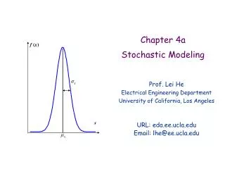
Chapter 4a Stochastic Modeling. Prof. Lei He Electrical Engineering Department University of California, Los Angeles URL: eda.ee.ucla.edu Email: lhe@ee.ucla.edu. f ( x ). σ x. x. μ x. Outline. Introduction to Stochastic Modeling Monte Carlo Simulation

E N D
Chapter 4aStochastic Modeling Prof. Lei He Electrical Engineering Department University of California, Los Angeles URL: eda.ee.ucla.edu Email: lhe@ee.ucla.edu f (x) σx x μx
Outline • Introduction to Stochastic Modeling • Monte Carlo Simulation • Example: SRAM cell Yield Estimation with MC&QMC
F (x) 1 f (x) dx 0 x x Review of Probability • R.V. X can take value from its domain randomly • Domain can be continuous/discrete, finite/infinite • PDF vs. CDF
f (x) σx x μx Review of Probability • Mean and Variance • Normal Distribution
Multivariate Distribution • Similar definition can be extended for multivariate cases • Joint PDF (JPDF), Covariance • Becomes much more complicated • Correlation MATTERS!!
Independent Random Variables Two events A and B are independent P(A ∩ B) = P(A)P(B). Two random variables X and Y are independent events A={X<=a} and B={Y<=b} are independent. For two independent variables X and Y, we have E[X Y] = E[X] E[Y] var(X + Y) = var(X) + var(Y),
Correlation Coefficient Normalized covariance: Always lies between -1 and 1 Correlation of 1 x ~ y, -1
Principal Component Analysis PAC helps tocompress and classify data It reduces thedimensionality of a data set (sample) by finding a new set of variables The new set has a smaller number of variables The new set nonetheless retains mostof the original information. By information we mean the variation present in the sample,given by the correlations between the original variables. The newvariables, called principal components (PCs), are uncorrelated, and areordered by the fraction of the total information each retains from high to low.
Geometric Interpretation of Principal Components A sample of n observations in the 2-D space x = (x1, x2) Goal:to account for the variation in a sample in as few variables as possible, to some accuracy
Geometric Interpretation of Principal Components • The1st PCz1 is a minimum distance fit to a line in x space • The2nd PCz2 is a minimum distance fit to a linein the plane • perpendicular to the 1st PC PCs are a series of linear least squares fits to a sample, each orthogonal to all the previous.
Outline • Introduction to Stochastic Modeling • Monte Carlo Simulation
Monte Carlo Simulation Problem Formulation Given a set of random variables X=(X1, X2, … Xn)T and a function of X, Y=f(X), estimate the distribution of the Y Method Generate N samples of X=(X1, X2, … Xn)T For each sample of X, calculate the correspondent sample of Y=f(X) Obtain the distribution of Y from the samples of Y
Advantage and Disadvantage of MC simulation Pro: Accurate Error→0 when N→∞ Flexible Works for any arbitrary distribution of X Works for any arbitrary function of f Simple Easy to implement Usually used as golden case in statistical analysis Con: Not efficient Need large N to obtain high accuracy Need to run large number of iterations Not suitable for statistical optimization
Example Given X1 and X2 are independent standard Gaussian RVs, estimate the distribution of max(X1, X2)
Quasi Monte Carlo Simulation Basic idea Use deterministic samples instead of pure random samples Select deterministic samples to cover the whole sample space evenly
Discrepancy Definition N is total number of samples, A(B, P) is the number of points in bounding box B, λs(B) is the volume of B Discrepancy measures how evenly the samples are in the sample place
Low Discrepancy Sequence Sample sequence with low discrepancy Low discrepancy array generation algorithms Faure sequence Neiderreiter sequence Sobol sequence Halton Sequence
Example: Halton Sequence Basic idea Choose a prime number as base (let's say 2) Write natural number sequence 1, 2, 3, ... in base Reverse the digits, including the decimal sign Convert back to base 10: 1 = 1.0 => 0.1 = 1/2 2 = 10.0 => 0.01 = 1/4 3 = 11.0 => 0.11 = 3/4 4 = 100.0 => 0.001 = 1/8 5 = 101.0 => 0.101 = 5/8 6 = 110.0 => 0.011 = 3/8 7 = 111.0 => 0.111 = 7/8 High dimensional array Use different base for different dimension Example 2-d array, X-base 2, y-base 3 1 => x=1/2 y=1/3 2 => x=1/4 y=2/3 3 => x=3/4 y=1/9 4 => x=1/8 y=4/9 5 => x=5/8 y=7/9 6 => x=3/8 y=2/9 7 => x=7/8 7=5/9
Advantage and Disadvantage of QMC Simulation Advantage Efficient Use fewer sample than random Monte Carlo simulation Disadvantage Only works in low dimension cases Very slow when number of random variations become large Not very common in statistical analysis
Comparison of MC and QMC QMC converges faster than MC
Reference • L. I. Smith. “A Tutorial on Principal Components Analysis”. Cornell University, USA, 2002. • Singhee, A., Rutenbar, R. “From Finance to Flip Flops: A study of Fast Quasi-Monte Carlo Methods from Computational Finance Applied to Statistical Circuit Analysis.”
Homework 5 • Yield Estimation using Monte Carlo Method • Consider “access time failure” : the time that voltage difference between BL_B and BL becomes larger than certain value. • The schematic are shown as below • Initial Value: • BL_B=1; Q_B=0; Q=1; BL=1; • Variation Source: • Vth (threshold voltage) of Mn1 and Mn2 • Leff of Mn1 and Mn2 • Device Model: • Use BSIM3 model for all MOSFETs
netlist • Netlist for 6-T cell SRAM • * SRAM netlist • Vdd dd 0 5 • Mn1 3 2 0 0 nmos • Mn2 3 5 4 4 nmos • Mn3 2 3 0 0 nmos • Mn4 2 5 1 1 nmos • Mp5 3 2 dd dd pmos • Mp6 2 3 dd dd pmos • all MOSFETs should use BSIM3 model
Detailed Steps • Performance Constraint: • The voltage difference between BL_B and BL should be larger than ∆v at the time-steptthresh. • Use Monte-Carlo and Quasi-Monte Carlo to calculate the yield Y, which is the percentage of circuits with satisfied performance. • Steps: • (1) Use MC and QMC to generate random sequences for two variable parameters with Matlab code. • (2) Perform transient simulations with these sequences, and compare the variable performance with constraint. • (3) Calculate the yield rate with definition. • Nominal Values, Performance Constraint and Matlab code will be provided soon • Due Feb 20th