Download
1 / 36
380 likes | 597 Views
Support Vector Machines (SVMs) Chapter 5 (Duda et al.). CS479/679 Pattern Recognition Dr. George Bebis. Learning through empirical risk minimization. Estimate g(x) from a finite set of observations by minimizing an error function, for example, the training error or empirical risk :.

E N D
Support Vector Machines (SVMs) Chapter 5 (Duda et al.) CS479/679 Pattern RecognitionDr. George Bebis
Learning through empirical risk minimization • Estimate g(x) from a finite set of observations by minimizing an error function, for example, the training error or empirical risk: class labels:
Learning through empirical risk minimization (cont’d) • Conventional empirical risk minimization over the training data does not imply good generalization to novel test data. • There could be several different functions g(x) which all approximate the training data set well. • Difficult to determine which function would have the best generalization performance.
Learning through empirical risk minimization (cont’d) Solution 1 Solution 2 Which solution is better?
Statistical Learning:Capacity and VC dimension • To guarantee good generalization performance, the capacity (i.e., complexity) of the learned functions must be controlled. • Functions with high capacity are more complicated (i.e., have many degrees of freedom). high capacity low capacity
Statistical Learning:Capacity and VC dimension (cont’d) • How do we measure capacity? • In statistical learning, the Vapnik-Chervonenkis (VC) dimension is a popular measure of capacity. • The VC dimension can predict a probabilistic upper bound on the test error (i.e., generalization error) of a classification model.
Statistical Learning:Capacity and VC dimension (cont’d) • A function that (1) minimizes the empirical risk and (2) has low VC dimension will generalize well regardless of the dimensionality of the input space: with probability(1-δ); (n: # of training examples) (Vapnik, 1995, “Structural Risk Minimization Principle”) structural risk minimization n
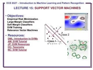
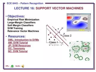
VC dimension and margin of separation • Vapnik has shown that maximizing the margin of separation between classes is equivalent to minimizing the VC dimension. • The optimal hyperplane is the one giving the largest margin of separation between the classes.
Margin of separation and support vectors • How is the margin defined? • The margin (i.e., empty space around the decision boundary) is defined by the distance to the nearest training patterns which we refer to as support vectors. • Intuitively speaking, these are the most difficult patterns to classify.
Margin of separation andsupport vectors (cont’d) different solutions corresponding margins
SVM Overview • SVMs perform structural risk minimization to achieve good generalization performance. • The optimization criterion is the margin of separation between classes. • Training is equivalent to solving a quadratic programming problem with linear constraints. • Primarily two-class classifiers but can be extended to multiple classes.
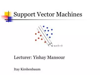
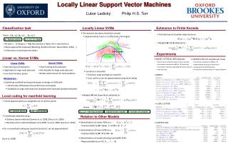
Linear SVM: separable case • Linear discriminant • Class labels • Normalized version Decide ω1if g(x) > 0 and ω2 if g(x) < 0
Linear SVM: separable case (cont’d) • The distance of a point xk from the separating hyperplane should satisfy the constraint: • To ensure uniqueness, we impose: • The above constraint becomes: (b is the margin)
Linear SVM: separable case (cont’d) quadratic programming problem maximize margin:
Linear SVM: separable case (cont’d) • Use Langrange optimization, we seek to minimize: • Easier to solve the “dual” problem (Kuhn-Tucker construction):
Linear SVM: separable case (cont’d) • The solution is given by: • It can be shown that if xk is not a support vector, then the corresponding λk=0. dot product Only support vectors affect the solution!
Linear SVM: non-separable case • Allow miss-classifications (i.e., soft margin classifier) by introducing positive error (slack) variables ψk :
Linear SVM: non-separable case (cont’d) • The constant c controls the trade-off between the margin and misclassification errors. • Aims to prevent outliers from affecting the optimal hyperplane.
Linear SVM: non-separable case (cont’d) • Easier to solve the “dual” problem (Kuhn-Tucker construction):
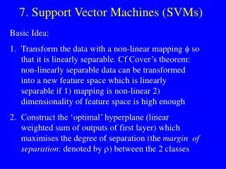
Nonlinear SVM • Extending these concepts to the non-linear case involves mapping the data to a high-dimensional space h: • Mapping the data to a sufficiently high dimensional space is likely to cast the data linearly separable in that space.
Nonlinear SVM (cont’d) Example:
Nonlinear SVM (cont’d) linear SVM: non-linear SVM:
Nonlinear SVM (cont’d) • The disadvantage of this approach is that the mapping might be very computationally intensive to compute! • Is there an efficient way to compute ? non-linear SVM:
The kernel trick • Compute dot products using a kernel function
The kernel trick (cont’d) • Comments • Kernel functions which can be expressed as a dot product in some space satisfy the Mercer’s condition (see Burges’ paper) • The Mercer’s condition does not tell us how to construct Φ() or even what the high dimensional space is. • Advantages of kernel trick • No need to know Φ() • Computations remain feasible even if the feature space has high dimensionality.
Polynomial Kernel K(x,y)=(x . y) d
Example (cont’d) h=6
Example (cont’d) (Problem 4)
Example (cont’d) w0=0
Example (cont’d) w =
Example (cont’d) w = The discriminant
Comments on SVMs • SVM is based on exact optimization, not on approximate methods (i.e., global optimization method, no local optima) • Appears to avoid overfitting in high dimensional spaces and generalize well using a small training set. • Performance depends on the choice of the kernel and its parameters. • Its complexity depends on the number of support vectors, not on the dimensionality of the transformed space.