Download
1 / 60
600 likes | 1.01k Views
Star Formation in Context. Neal Evans University of Texas at Austin. Context. Individual star formation in detail Initial conditions and early evolution Formation and evolution of disks Provides the context for planet formation Massive, clustered star formation Details less accessible

E N D
Star Formation in Context Neal Evans University of Texas at Austin
Context • Individual star formation in detail • Initial conditions and early evolution • Formation and evolution of disks • Provides the context for planet formation • Massive, clustered star formation • Details less accessible • Statistical results • Context for galaxy formation and evolution
Low-mass Star Formation Features: Dusty envelope Rotation Disk Bipolar outflow R. Hurt, SSC
Science Goals • Complete database for nearby (< 350 pc) regions • Low mass star and substar formation • Follow evolution: starless cores to planet-forming disks • Coordinate with FEPS team • ensure complete coverage of 0 to 1 Gyr • Cover range of other variables • mass, rotation, turbulence, environment, … • separate these from evolution.
A Typical Starless Core L1014 distance ~ 200 pc, but somewhat uncertain. R-band image;dust blocks stars behind and our view of what goes on inside.
Forming Star Seen in Infrared Three Color Composite: Blue = 3.6 microns Green = 8.0 microns Red = 24 microns R-band image from DSS at Lower left. We see many stars through the cloud not seen in R. The central source is NOT a background star. L1014 is forming a star (or substar) C. Young et al. ApJS, 154, 396
JHK Image J, H, K Image of L1014 KPNO 4-m + Flamingos J (19.7) H(20.9) K(19.4) Huard et al. in prep. Preliminary reduction Faint conical nebula to north with apex on IRAC source. BIMA peak to south likely obscures southern lobe. Not a background source.
Lessons from L1014 • “Starless” cores may not be • Or may have substellar objects • Very low luminosity sources may exist • Must be low mass and low accretion • Very compact outflow detected with SMA • Peculiar, non-thermal radio source • Early, small disks are easily detected • Md ~ 4 x 10⁻⁴ Msun (Rd/50AU)0.5 • Easily detected (SNR = 50–100) • Rd ~ 50 AU • Are there others? • About 15 candidates
Detailed Studies of Low Mass Star Formation • Isolation • Nearby • Good spatial resolution • Can study faint features • Predictive theories exist • n( r), v( r) • With caveats, L(t) • Allows one to calculate T(r)
We need a self-consistent model • All quantities vary along line of sight • Dust temperature, Td( r) • Heating from outside, later inside • Gas temperature, TK( r) • Gas-dust collisions, CRs, PE heating • Density, n(r), variations predicted, observed • Velocity, v(r), variations predicted, observed • Abundance, X(r), variations predicted, observed • Photodissociation, freeze-out, desorption
An Evolutionary Model • Assume a slow approach to collapse • Sequence of Bonnor-Ebert spheres • From nc = 104 to 107 in 6 steps of factors of 3 • Total time 1 million years • Time step shrinks by factor of 2 for each step in nc • Embedded in cloud with AV = 0.5 (or 3) mag • Approach a singular isothermal sphere • Initiate collapse at t =0 • Inside-out collapse (Shu) • At each time step, calculate: • n (r), v(r), L, Td(r), TK(r), X(r) • Chemistry follows gas parcels during collapse • The radiation field, density, temperature change as it falls
Theory gives n(r,t), v(r,t) C. Young
L(t) from Accretion, Contraction L(t) calculated. First accretion. First onto large (5 AU) surface (first hydrostatic core). Then onto PMS star with R = 3 Rsun, after 20,000 to 50,000 yr. And onto disk. Prescriptions from Adams and Shu. Contraction luminosity and deuterium burning dominates after t ~100,000 yr. C. Young and Evans, submitted.
Dust Radiative Transport Use DUSTY to compute Td( r, t). Include interstellar radiation and central heating from L(t). Compute SED and radial profile from DUSTY and obssphere. C. Young and Evans, submitted
Calculate Gas Temperature J. Lee et al. 2004 Use gas energetics code (Doty) with gas-dust collisions, cosmic rays, photoelectric heating, gas cooling. Calculate TK( r, t).
Calculate Abundances Chemical code by E. Bergin 198 time steps of varying length, depending on need. Medium sized network with 80 species, 800 reactions. Follows 512 gas parcels. Includes freeze-out onto grains and desorption due to thermal, CR, photo effects. No reactions on grains. Assume binding energy on silicates for this case. J. Lee et al. 2004
A Closer Look A few abundance profiles at t=100,000 yr. Vertical offset for convenience (except CO and HCN). Big effect is CO desorption, which affects most other species. Secondary peaks related to evaporation of other species. J. Lee et al. 2004
Calculate Observables Line profiles calculated from Monte Carlo plus virtual telescope codes. Includes collisional excitation, trapping. Variations in density, temperature, abundance, velocity are included. Assumes distance of 140 pc and typical telescope properties. J. Lee et al. 2004 J. Lee et al. In prep
A Closer Look Lines of HCO+ (J = 1–0 and 3–2). Shown for four times and for different amounts of extinction in the surrounding medium. Blue profiles are indicative of collapse. J. Lee et al. 2004
Dynamical vs Static Models Previous chemical models did not include dynamical evolution. A fully dynamical model captures the changing density and temperature of a gas parcel. J. Lee et al. 2005, in prep.
Abundances Differ Solid curve show result of dynamical model; dashed is static model. In particular, the peaks at small radii from direct evaporation of the molecule are missed by static models. J. Lee et al. 2005, in prep.
Consequences for Line Profiles J. Lee et al. 2005, in prep.
Comparison to Observations Observations of B335 Three CS transitions Red line is from chemical model. Evans et al. 2005, submitted
HCN in B335 and Model Evans et al. 2005, submitted
3D vs 1D Dust Models 3D Dust radiative transfer: Allows modeling of shape. Application to L1544. Overall results similar to 1D. Nice constraint on internal luminosity from shape of contours. Doty et al. 2005, MNRAS, in press
Summary so far • Beginning to develop evolutionary models • Self-consistent physical, chemical models • Get a feel for what parameters affect what • Starting to explore 3D models • Chemistry is crucial to physical modeling • Conclusions about dynamics from lines depend on X(r) • Surrounding cloud/external radiation important • Future work • Change dust opacities when ices evaporate • Check effect of chemistry on energetics • Try other dynamical models
Star Formation in Larger Clouds • Where do stars form in large molecular clouds? • Early evidence indicated only in dense gas • Lada et al. 1991: Study of L1630 • But surveys were incomplete • Need to survey at longer wavelengths • Large cloud surveys with c2d and COMPLETE
Perseus 12CO Map The COMPLETE Team; Ridge et al.in prep.
Perseus 1mm Continuum M. Enoch et al., in prep.
Perseus 13CO The COMPLETE Team; Ridge et al.in prep.
Perseus MIPS (24+70) Stapelfeldt et al. in prep.
Perseus Zoom IRAC1 (blue), IRAC3(green, MIPS1(red)
Complementary Millimeter & Spitzer IRAC/MIPS Observations: B1 in Perseus Bolocam 1mm MIPS 24 m Enoch et al. in prep. Dark blue: 24; light blue 70 microns
Lessons from Perseus • There are interesting things going on outside the famous regions • Large surveys needed to remove bias • A panchromatic view is needed • Molecular emission • Different molecules show different things • Dust continuum emission (across wavelengths) • Locations, L, etc. of forming stars • Much analysis remains to be done…
Disk Evolution • Do all solar-mass stars have disks? • Do weak-line T Tauri stars have debris disks? • Are there variables besides time? • What are the timescales for disk evolution? • Formation and early evolution during collapse • How does the transition from accretion disks to debris disks depend on time and other factors? • What is the structure of disks? • What is the chemistry in disks?
Evidence for large inner rims in cTTs The solid blue line (Total SED A) corresponds to the total SED when the inner rim is irradiated only by the photosphere of the central star (rim A). The solid red line (Total SED B) corresponds to the total SED when the emission from the inner rim is scaled by a factor W. W ranges from ~ 1 to ~7. The inner rim is powered by more than the stellar photosphere Missing source of energy? UV radiation from the accretion shock cgplus model (Dullemond et al. 2001) ~ 3.5 RrimA~ 0.04 AU RrimA~ 0.07 AU Cieza et al. in prep.
Finding disks with MIPS Model has 0.1 Mmoon of 30 mm size dust grains in a disk from 30–60 AU Bars are 3 s Model based on disks around A stars
A New Disk in Cha II • One source not previously identified as a YSO on K vs. K-24 plot • Factor of 3 excess in 24 micron flux over stellar model indicating the presence of a disk K.Young et al. in prep.
24mm Excesses vs Age decay over ~ 200 Myr - many stars of all ages have no, or very little excess.
Chemistry in Disks Robert Hurt, SSC
Studies of High Mass Regions • Many Detailed Studies • Ho, Zhang, Keto, … • Surveys • van der Tak et al. (2000) (14 sources) • Beuther et al. (2002) (69 sources) • Survey of water masers for CS • CS survey Plume et al. (1991, 1997) • Dense: <log n> = 5.9 • Maps of 51 in 350 micron dust emission • Mueller et al. 2002 • Maps of 63 in CS J = 5–4 emission • Shirley et al. 2003
Luminosity versus Mass Log Luminosity vs. Log M red line: masses of dense cores from dust Log L = 1.9 + log M blue line: masses of GMCs from CO Log L = 0.6 + log M L/M much higher for dense cores than for whole GMCs. Mueller et al. (2002)
Linewidth versus Size Correlation is weak. Linewidths are 4-5 times larger than in samples of lower mass cores. Massive clusters form in regions of high turbulence, pressure. Shirley et al. 2003
Cumulative Mass Function Incomplete below 103 Msun. Fit to higher mass bins gives slope of about –0.93. Steeper than that of CO clouds or clumps (–0.5 on this plot). Similar to that of clusters, associations (Massey et al. 1995) in our Galaxy and in Antennae (Fall et al. 2004). Shirley et al. 2003
Hints of Dynamics A significant fraction of the massive core sample show self-reversed, blue-skewed line profiles in lines of HCN 3-2. Of 18 double-peaked profiles, 11 are blue, 3 are red. Suggests inflow motions of overall core. Vin ~ 1 to 4 km/s over radii of 0.3 to 1.5 pc. J. Wu et al. (2003)
Low Mass vs. High Mass • Low Mass star formation • “Isolated” (time to form < time to interact) • Low turbulence (less than thermal support) • Slow infall • Nearby (~ 100 pc) • High Mass star formation • “Clustered” • Time to form may exceed time to interact • Turbulence >> thermal • Fast infall? • More distant (>400 pc)