Download
1 / 41
410 likes | 764 Views
Modeling Software Systems Lecture 2 Book: Chapter 4 Systems of interest Sequential systems. Concurrent systems. Distributive systems. Reactive systems. Embedded systems (software + hardware). Sequential systems. Perform some computational task.

E N D
Modeling Software Systems Lecture 2 Book: Chapter 4
Systems of interest • Sequential systems. • Concurrent systems. • Distributive systems. • Reactive systems. • Embedded systems (software + hardware).
Sequential systems. • Perform some computational task. • Have some initial condition, e.g.,0≤i≤n A[i]≥0, A[i] integer. • Have some final assertion, e.g.,0≤i≤n-1 A[i]<A[i+1].(What is the problem with this spec?) • Are supposed to terminate.
Concurrent Systems Involve several computation agents. Termination may indicate an abnormal event (interrupt, strike). May exploit diverse computational power. May involve remote components. May interact with users (Reactive). May involve hardware components (Embedded).
Problems in modeling systems • Representing concurrency:- Allow one transition at a time.- Allow coinciding transitions.- Allow a partial order between events. • Granularity of transitions. • Execution model (linear, branching). • Global or local states.
Modeling • V={v0,v1,v2, …} - a set of variables, over some domain. • p(v0, v1, …, vn) - a parametrized assertion, e.g., v0=v1+v2/\v3>v4. • A state is an assignment of values to the program variables. For example: s=<v0=1,v2=3,v3=7,…,v18=2> • p(s) is p under the assignment s.
State space • The state space of a program is the set of all possible states for it. • For example, if V={a, b, c} and the variables are over the naturals, then the state space includes: <a=0,b=0,c=0>,<a=1,b=0,c=0>, <a=1,b=1,c=0>,<a=932,b=5609,c=6658>…
Atomic Transitions • Each atomic transition represents a small peace of code such that no smaller peace of code is observable. • Is a:=a+1 atomic? • In some systems, e.g., when a is a register and the transition is executed using an inc command.
Execute the following when x=0 in two concurrent processes: P1:a=a+1 P2:a=a+1 Result: a=2. Is this always the case? Consider the actual translation: P1:load R1,a inc R1 store R1,a P2:load R2,a inc R2 store R2,a a may be also 1. Non atomicity
Representing transitions • Each transition has two parts: • The enabling condition: a predicate. • The transformation: a multiple assignment. • For example:a>b (c,d):=(d,c)This transition can be executed in states where a>b. The result of executing it isswitching the value of c with d.
Initial condition • A predicate p. • The program can start from states s such that p(s) holds. • For example:p(s)=a>b /\ b>c.
A transition system • A (finite) set of variables V over some domain(s). • A set of states S. • A (finite) set of transitions T, each transition et has • an enabling condition e, and • a transformation t. • An initial condition p.
Example • V={a, b, c, d, e}. • S: all assignments of natural numbers for variables in V. • T={c>0(c,e):=(c-1,e+1), d>0(d,e):=(d-1,e+1)} • p: c=a /\ d=b /\ e=0 • What does this transition relation do?
The interleaving model • An execution is a finite or infinite sequence of states s0, s1, s2, … • The initial state satisfies the initial condition, I.e., p(s0). • Moving from one state si to si+1 is by executing a transition et: • e(si), I.e., sisatisfies e. • si+1 is obtained by applying t to si.
Example: • s0=<a=2, b=1, c=2, d=1, e=0> (satisfies the initial condition) • s1=<a=2, b=1, c=1, d=1, e=1>(first transition executed) • s2=<a=2, b=1, c=1, d=0, e=2>(second transition executed) • s3=<a=2, b=1 ,c=0, d=0, e=3>(first transition executed again)
Temporal Logic (informal) • First order logic or propositional assertions describe a state. • Modalities: • <>p means p will happen eventually. • []p means p will happen always. p p p p p p p p
More temporal logic • We can construct more complicated formulas: []<>p -- It is always the case that p will happen again in the future (infinitely often). <>p /\ <>q -- Both p and q will happen in the future, the order between them not determined. • The property must hold for all the executions of the program.
L0:While True do NC0:wait(Turn=0); CR0:Turn=1 endwhile || L1:While True do NC1:wait(Turn=1); CR1:Turn=0 endwhile T0:PC0=L0PC0:=NC0 T1:PC0=NC0/\Turn=0 PC0:=CR0 T2:PC0=CR0 (PC0,Turn):=(L0,1) T3:PC1=L1PC1=NC1 T4:PC1=NC1/\Turn=1 PC1:=CR1 T5:PC1=CR1 (PC1,Turn):=(L1,0) The transitions Initially: PC0=L0/\PC1=L1
Turn=1 L0,L1 Turn=0 L0,L1 Turn=0 L0,NC1 Turn=0 NC0,L1 Turn=1 L0,NC1 Turn=1 NC0,L1 Turn=0 NC0,NC1 Turn=0 CR0,L1 Turn=1 L0,CR1 Turn=1 NC0,NC1 Turn=0 CR0,NC1 Turn=1 NC0,CR1 The state space
Turn=0 L0,L1 Turn=1 L0,L1 Turn=0 L0,NC1 Turn=0 NC0,L1 Turn=1 L0,NC1 Turn=1 NC0,L1 Turn=0 NC0,NC1 Turn=0 CR0,L1 Turn=1 L0,CR1 Turn=1 NC0,NC1 Turn=0 CR0,NC1 Turn=1 NC0,CR1 []¬(PC0=CR0/\PC1=CR1)
Turn=0 L0,L1 Turn=1 L0,L1 Turn=0 L0,NC1 Turn=0 NC0,L1 Turn=1 L0,NC1 Turn=1 NC0,L1 Turn=0 NC0,NC1 Turn=0 CR0,L1 Turn=1 L0,CR1 Turn=1 NC0,NC1 Turn=0 CR0,NC1 Turn=1 NC0,CR1 [](Turn=0--><>Turn=1)
Turn=0 L0,L1 Turn=0 L0,NC1 Turn=1 L0,NC1 Turn=0 NC0,NC1 Turn=1 L0,CR1 Turn=0 CR0,NC1 Interleaving semantics
Turn=0 L0,L1 Turn=0 L0,L1 Turn=0 L0,NC1 Turn=0 L0,NC1 Turn=1 L0,NC1 Turn=0 NC0,NC1 Turn=1 L0,CR1 Turn=0 CR0,NC1 Interleaving semantics
Turn=0 L0,L1 Turn=0 L0,NC1 Turn=0 NC0,L1 Turn=1 L0,NC1 Turn=0 NC0,NC1 Turn=0 NC0,NC1 Turn=0 CR0,L1 Turn=0 CR0,NC1 Turn=0 CR0,NC1 Turn=0 CR0,NC1 An unfolding
Partial Order Semantics • Sometimes called “real concurrency”. • There is no total order between events. • More intuitive. Closer to the actual behavior of the system. • More difficult to analyze. • Less verification results. • Natural transformation between models. • Partial order: (S , <), where < is • Reflexive: x<y /\ y<z x<z. • Antisymmetric: for no x, y, x<y /\ y>x. • Antireflexive: for no x, x<x.
Bank Example • Two branches, initially $1M each. • In one branch: deposit, $2M. • In another branch: robbery. • How to model the system?
Global state space $1M, $1M deposit robbery $3M, $1M $1M, $0M robbery $3M, $0M deposit
Should we invest in this bank? $1M, $1M Invest! deposit robbery $3M, $1M $1M, $0M robbery $3M, $0M deposit Do not Invest! Invest!
Partial Order Description $1M $1M deposit robbery $3M $0M
Constructing global states $1M $1M deposit robbery $3M $0M
pc1=m0,x=0 pc2=n0,y=0,z=0 m0 m0:x:=x+1 n0:ch?z pc1=m1,x=1 m1 n0 P1 P2 pc2=n1,y=0,z=1 pc1=m0,x=1 m1:ch!x n1:y:=y+z n1 m0 pc1=m1,x=2 pc2=n0,y=1,z=1 m1 n0 pc1=m0,x=2 pc2=n1,y=1,z=2 m0 n1 Modeling with partial orders
Linearizations pc1=m0,x=0 pc2=n0,y=0,z=0 m0 pc1=m0,x=0,pc2=n0,y=0,z=0 pc1=m1,x=1 pc1=m1,x=1,pc2=n0,y=0,z=0 m1 n0 pc1=m0,x=1,pc2=n1,y=0,z=1 pc2=n1,y=0,z=1 pc1=m0,x=1 pc1=m1,x=2,pc2=n1,y=0,z=1 m0 n1 pc1=m1,x=2,pc2=n0,y=1,z=1 pc1=m1,x=2 pc2=n0,y=1,z=1 pc1=m0,x=2,pc2=n1,y=1,z=2 m1 n0 pc1=m0,x=2 pc2=n1,y=1,z=2 m0 n1
Linearizations pc1=m0,x=0 pc2=n0,y=0,z=0 m0 pc1=m0,x=0,pc2=n0,y=0,z=0 pc1=m1,x=1 pc1=m1,x=1,pc2=n0,y=0,z=0 m1 n0 pc1=m0,x=1,pc2=n1,y=0,z=1 pc2=n1,y=0,z=1 pc1=m0,x=1 pc1=m0,x=1,pc2=n0,y=1,z=1 n1 m0 pc1=m1,x=2,pc2=n0,y=1,z=1 pc1=m1,x=2 pc2=n0,y=1,z=1 pc1=m0,x=2,pc2=n1,y=1,z=2 m1 n0 pc1=m0,x=2 pc2=n1,y=1,z=2 m0 n1
Bank with one teller $1M $1M deposit deposit robbery $3M $1.1M $0M deposit deposit $3.1M
Partial order execution 1 $1M $1M deposit robbery $3M $0M deposit $3.1M
Partial order execution 2 $1M $1M deposit robbery $1.1M $0M deposit $3.1M
L0:While True do NC0:wait(Turn=0); CR0:Turn=1 endwhile || L1:While True do NC1:wait(Turn=1); CR1:Turn=0 endwhile T0:PC0=L0PC0:=NC0 T1:PC0=NC0/\Turn=0PC0:=CR0 T1’:PC0=NC0/\Turn=1PC0:=NC0 T2:PC0=CR0(PC0,Turn):=(L0,1) T3:PC1==L1PC1=NC1 T4:PC1=NC1/\Turn=1PC1:=CR1 T4’:PC1=NC1/\Turn=0PC1:=N1 T5:PC1=CR1(PC1,Turn):=(L1,0) Bust waiting Initially: PC0=L0/\PC1=L1
Turn=0 L0,L1 Turn=1 L0,L1 Turn=0 L0,NC1 Turn=0 NC0,L1 Turn=1 L0,NC1 Turn=1 NC0,L1 Turn=0 NC0,NC1 Turn=0 CR0,L1 Turn=1 L0,CR1 Turn=1 NC0,NC1 Turn=0 CR0,NC1 Turn=1 NC0,CR1 [](Turn=0--><>Turn=1)
Fairness Restriction on the set of ‘legal’ sequences. • Weak process fairness: if some process is enabled continuously from some state, it will be executed. • Weak transition fairness: if some transition is enabled continuously from some state, it will be executed. • Strong process fairness: if some process is enabled infinitely often, it will be executed (infinitely often). • Strong transition fairness: if some transition is enabled infinitely often, then it will be executed.
P1::x:=1 P2::while y=0 do [z:=z+1 [] if x=1 then y:=1] end while Example Initially: x=0 /\ y=0 /\ z=0 /\pc1=l0 /\ pc2=r0 Termination? Termination of P1? No fairness?. Nothing guaranteed Weak transition (process) fairness? P1 terminates Strong process fairness? P1 terminates. Strong transition fairness? P1 and P2 terminate.
φ ψ Hierarchy of fairness assumptions Strong transition If φ holds then also ψ. If a sequence is fair w.r.t. φ it is also fair w.r.t. Ψ. A system which assumes φhas no more executions than one assuming Ψ Strong process weak transition weak process