Download
1 / 171
1.82k likes | 2.9k Views
Meshfree Methods and Simulations of Material Failures Shaofan Li Department of Civil and Environmental Engineering, University of California at Berkeley Collaborators Dr. Bo C Simonsen, Technical University of Denmark; Dr. Daniel C. Simkins,

E N D
Meshfree Methods and Simulations of Material Failures ShaofanLi Department of Civil and Environmental Engineering, University of California at Berkeley
Collaborators Dr. Bo C Simonsen, Technical University of Denmark; Dr. Daniel C. Simkins, University of South Florida; Dr. Sergey N. Medyanik, Northwestern University
Table of Contents • Introduction: What is Meshfree Method • Simulations of Large Deformations • Simulations of Strain Localizations • Simulations of Dynamics Shear Band Propagations • Simulations of Ductile Fracture 6. Simulations of Impact and penetrations 7. Conclusions
I. Introduction of meshfree methods Mesh vs. Meshfree
Meshfree Methods • Smooth Particle Hydrodynamics (SPH) • Element Free Galerkin (EFG) • Reproducing Kernel Particle Method (RKPM) 1. Unknown is represented by convolving a smooth kernel with dependent variable 2. Discretize by evaluating integral via nodal integration
RKPM Kernel • f(x-y) is a smooth compactly-supported function, e.g. cubic spline • PT(x) = [1 x y z xy xz …] is vector of monomial terms • b(x) (called the normalizer) is used to regain discrete partition of unity
Moment Equation Note and P(0) = (1, 0, 0, …, 0) then
By Taylor theorem, therefore
Compare FEM shape function with Meshfree shape function (a) FEM ; (b) Meshfree
Compare FEM shape function with Meshfree shape function (a) FEM ; (b) Meshfree
(a) Shape function (b) Derivative (c) Derivative (d) Derivative “The Cloud”: 3-D Meshfree shape function and its first derivatives generated by the tri-linear polynomial basis, P(X) = (1, x1 ,x2 , x3 , x1x2 ,x2x3 , x3x1 , x1x2x3 )
1.2 A Few Virtues of Meshfree Methods Convergence Property as as Reproducing Property For That is Non-local Interpolation (Discrete Convolution)
* Large Support Size It enables meshfree discretization/interpolation to endure large mesh distortion and sustain computation without remeshing; is deformation map
Example 2.1 : Compression of A Rubber Cylinder FEMMeshfree 50% Compression 65% Compression 85% Compression 90% Compression
Example 2.2 A pinched cylindrical shell Material Properties Computational Parameters Number of Particles: 30300 Time Step:
Deformation Sequence of A Pinched Cylinder (a) (b) (c) (c) (d) (e)
Example 2.3 Hemispheric Shell with Pinched Load Summary: Material: Elastic-plastic material; Geometry: Hemisphere shell with radius of 1 inch, thickness of 0.04 inch. Particles: 12,300
(c) t = 3.010-3s (b) t = 1.510-3s (a) t = 0.510-3s (f) t = 7.510-3s (d) t = 4.510-3s (e) t = 6.010-3s
Example 2.4 The snap-through of a conic shell Material Properties Computational Parameters Number of Particles: 12300 Time Step:
The snap-through of a 3D conic shell (a) (b) (c) (c) (d) (e)
Excessive mesh distortion (hourglassing) ABAQUS/Explicit RKPM/Explicit
Meshfree Simulation of Strain Localization Hardening Softening From Reid, Gilbert, and Hahn [1966]
Meshfree Methods: Element-free Galerkin (EFG) Fleming and Belytechko [1997]
Shearband Path for a Plate with 31 Holes (FEM vs. Meshfree Methods) (b) 60 90 mesh (c) 90 60 mesh (a) 60 60 mesh (d) 60 90 particles (e) 90 60 particles (c) 60 60 particles
FEM Meshfree (a) 20 20 (b) 30 20 (c) 40 20 (d) 50 20
4. Meshfree Multiscale Computations = Scale 0 + Scale 1 + Scale 2 + …... 1-D Meshfree Multiscale Basis Functions for Polynomial Basis P = ( 1, x, x2, x3 )
[0,0] [1,0] [0,1] [2,0] [1,1] [0,2] Hierarchical Partition of Unity of Quadratic Basis
Multiscale Analysis Spectral Meshfree Adaptive Simulations
Multiscale Analysis (a) Total Scale(b) Low Scale(c ) High Scale(d) Adaptive Pattern Total Particles: 3321 Particles used for adaptive calculation: 361
Example 4.2 Multiresolution Analysis Total Scale Low Scale High Scale
Tension of A Bar with A Hole Meshfree (particles) Zoom in Kinematically Admissible Mode I 4272 particles/layer with 3 layers in thickness direction Mesh-based (element distortion)
Symmetry slip line solution Shear Plane Development for a bar with A Hole in Tension (I)
How to simulate curve shearband Curved Shear Band Formation in Double-Notched Bar in Tension 13364 particles Reference 1: Ewing, D.J.F. and Hill, R. J. Mech. Phys. Solids, 15, 115 (1967)