Download
1 / 50
500 likes | 618 Views
OR/MA 504 Chapter 4 Network Modeling. Introduction to Mathematical Programming. Introduction. A large variety of linear programming applications can be represented graphically as networks. This chapter focuses on several such problems: Transshipment Problems Shortest Path Problems

E N D
OR/MA 504Chapter 4Network Modeling Introduction to Mathematical Programming
Introduction • A large variety of linear programming applications can be represented graphically as networks. • This chapter focuses on several such problems: • Transshipment Problems • Shortest Path Problems • Maximal Flow Problems • Transportation/Assignment Problems • Generalized Network Flow Problems • The Minimum Spanning Tree Problem
Network Flow Problem Characteristics • Network flow problems can be represented as a collection of nodes connected by arcs. • There are three types of nodes: • Supply • Demand • Transshipment • We’ll use negative numbers to represent supplies and positive numbers to represent demand.
A Transshipment Problem:The Bavarian Motor Company +100 $30 Boston $50 2 -200 Newark 1 Columbus +60 $40 3 $40 $35 Richmond $30 +80 Atlanta 4 +170 5 $25 $50 $45 $35 Mobile +70 J'ville -300 6 $50 7
Defining the Decision Variables For each arc in a network flow model we define a decision variable as: Xij = the amount being shipped (or flowing) from node ito node j For example… X12 = the # of cars shipped from node 1 (Newark) to node 2 (Boston) X56 = the # of cars shipped from node 5 (Atlanta) to node 6 (Mobile) Note: The number of arcs determines the number of variables!
Defining the Objective Function Minimize total shipping costs. MIN: 30X12 + 40X14 + 50X23 + 35X35 +40X53 + 30X54 + 35X56 + 25X65 + 50X74 + 45X75 + 50X76
Constraints for Network Flow Problems:The Balance-of-Flow Rules For Minimum Cost Network Apply This Balance-of-Flow Flow Problems Where: Rule At Each Node: Total Supply > Total Demand Inflow-Outflow >= Supply or Demand Total Supply < Total Demand Inflow-Outflow <=Supply or Demand Total Supply = Total Demand Inflow-Outflow = Supply or Demand
Defining the Constraints • In the BMC problem: Total Supply = 500 cars Total Demand = 480 cars • For each node we need a constraint like this: Inflow - Outflow >= Supply or Demand • Constraint for node 1: –X12 – X14 >= – 200(Note: there is no inflow for node 1!) • This is equivalent to: +X12 + X14 <= 200 (Supply >= Demand)
Defining the Constraints • Flow constraints –X12 – X14 >= –200 } node 1 +X12 – X23 >= +100 } node 2 +X23 + X53 – X35 >= +60 } node 3 + X14 + X54 + X74 >= +80 } node 4 + X35 + X65 + X75 – X53 – X54 – X56 >= +170} node 5 + X56 + X76 – X65 >= +70 } node 6 –X74 – X75 – X76 >= –300 } node 7 • Nonnegativity conditions Xij >= 0 for allij
Implementing the Model See file Fig4-1.xls
120 20 80 40 210 70 Optimal Solution to the BMC Problem +100 $30 Boston $50 2 -200 Newark 1 Columbus +60 $40 3 $40 Richmond +80 Atlanta 4 +170 5 $45 Mobile +70 J'ville -300 6 $50 7
The Shortest Path Problem • Many decision problems boil down to determining the shortest (or least costly) route or path through a network. • Ex. Emergency Vehicle Routing • This is a special case of a transshipment problem where: • There is one supply node with a supply of -1 • There is one demand node with a demand of +1 • All other nodes have supply/demand of +0
The American Car Association +0 3.3 hrs +1 L'burg 5 pts 9 Va Bch 11 5.0 hrs 9 pts 2.0 hrs 4 pts 4.7 hrs 2.7 hrs +0 9 pts +0 4 pts 1.1 hrs K'ville 3 pts G'boro Raleigh 5 2.0hrs 3.0 hrs 8 9 pts 10 4 pts +0 1.7 hrs 5 pts A'ville 1.5 hrs +0 6 2.3 hrs 3 pts +0 3 pts Chatt. 2.8 hrs 7 pts 3 Charl. 2.0 hrs 7 8 pts +0 1.7 hrs 3.0 hrs 4 pts 4 pts 1.5 hrs G'ville 2 pts 4 Atlanta +0 B'ham 2.5 hrs 2 3 pts 1 2.5 hrs +0 3 pts -1
Solving the Problem • There are two possible objectives for this problem • Finding the quickest route (minimizing travel time) • Finding the most scenic route (maximizing the scenic rating points) See file Fig4-2.xls
The Equipment Replacement Problem • The problem of determining when to replace equipment is another common business problem. • It can also be modeled as a shortest path problem…
The Compu-Train Company • Compu-Train provides hands-on software training. • Computers must be replaced at least every two years. • Two lease contracts are being considered: • Each requires $62,000 initially • Contract 1: • Prices increase 6% per year • 60% trade-in for 1 year old equipment • 15% trade-in for 2 year old equipment • Contract 2: • Prices increase 2% per year • 30% trade-in for 1 year old equipment • 10% trade-in for 2 year old equipment
+0 +0 $63,985 4 2 $30,231 $33,968 $28,520 $32,045 +1 5 1 3 -1 $67,824 $60,363 +0 Network for Contract 1 Cost of trading after 1 year: 1.06*$62,000 - 0.6*$62,000 = $28,520 Cost of trading after 2 years: 1.062*$62,000 - 0.15*$62,000 = $60,363 Cost of trading in year 2 after trading in year 1: 1.062*$62,000 – 0.6(1.06*$62,000) = $69,663 - $39,432 = $30,231
Solving the Problem See file Fig4-3.xls
Processing Plants Groves Distances (in miles) Supply Capacity 21 Mt. Dora Ocala 200,000 275,000 1 4 50 40 35 30 Eustis Orlando 600,000 400,000 2 5 22 55 20 Clermont Leesburg 225,000 300,000 3 6 25 Transportation & Assignment Problems • Some network flow problems don’t have trans-shipment nodes; only supply and demand nodes. These problems are implemented more effectively using the technique described in Chapter 2.
Generalized Network Flow Problems • In some problems, a gain or loss occurs in flows over arcs. • Examples • Oil or gas shipped through a leaky pipeline • Imperfections in raw materials entering a production process • Spoilage of food items during transit • Theft during transit • Interest or dividends on investments • These problems require some modeling changes.
Coal Bank Hollow Recycling Process 1 Process 2 Material Cost Yield Cost Yield Supply Newspaper $13 90% $12 85% 70 tons Mixed Paper $11 80% $13 85% 50 tons White Office Paper $9 95% $10 90% 30 tons Cardboard $13 75% $14 85% 40 tons Newsprint Packaging Paper Print Stock Pulp Source Cost Yield Cost Yield Cost Yield Recycling Process 1 $5 95% $6 90% $8 90% Recycling Process 2 $6 90% $8 95% $7 95% Demand 60 tons 40 tons 50 tons
Network for Recycling Problem -70 Newspaper $13 1 $12 Newsprint 95% +0 +60 90% pulp 7 $5 80% $11 Recycling 90% Mixed -50 Process 1 paper $6 95% 5 2 $13 $8 90% 75% Packing +40 paper pulp $9 8 95% 85% White 85% -30 office $6 paper $10 Recycling 90% 3 $8 90% Process 2 Print $7 6 +50 stock 85% 95% $13 pulp +0 9 -40 Cardboard $14 4
Defining the Objective Function Minimize total cost. MIN: 13X15 + 12X16 + 11X25 + 13X26 + 9X35+ 10X36 + 13X45 + 14X46 + 5X57 + 6X58 + 8X59 + 6X67 + 8X68 + 7X69
Defining the Constraints-I • Raw Materials -X15 -X16 >= -70 } node 1 -X25 -X26 >= -50 } node 2 -X35 -X36 >= -30 } node 3 -X45 -X46 >= -40 } node 4
Defining the Constraints-II • Recycling Processes +0.9X15+0.8X25+0.95X35+0.75X45- X57- X58-X59 >= 0 } node 5 +0.85X16+0.85X26+0.9X36+0.85X46-X67-X68-X69 >= 0 } node 6
Defining the Constraints-III • Paper Pulp +0.95X57 + 0.90X67 >= 60 } node 7 +0.90X57 + 0.95X67 >= 40 } node 8 +0.90X57 + 0.95X67 >= 50 } node 9
Implementing the Model See file Fig4-4.xls
Important Modeling Point • In generalized network flow problems, gains and/or losses associated with flows across each arc effectively increase and/or decrease the available supply. • This can make it difficult to tell if the total supply is adequate to meet the total demand. • When in doubt, it is best to assume the total supply is capable of satisfying the total demand and use Solver to prove (or refute) this assumption.
The Maximal Flow Problem • In some network problems, the objective is to determine the maximum amount of flow that can occur through a network. • The arcs in these problems have upper and lower flow limits. • Examples • How much water can flow through a network of pipes? • How many cars can travel through a network of streets?
The Northwest Petroleum Company Pumping Pumping Station 3 Station 1 3 4 2 6 2 6 Oil Field 1 6 Refinery 2 4 4 5 3 5 Pumping Pumping Station 2 Station 4
Max Flow Problem Set-Up • Solve as transshipment problem: • Add return arc from ending node to the starting node • Assign demand of 0 to all nodes in network • Maximize flow over the return arc
The Northwest Petroleum Company Pumping Pumping Station 3 Station 1 +0 +0 3 4 2 6 2 6 +0 +0 Oil Field 1 6 Refinery 2 4 4 5 3 +0 5 +0 Pumping Pumping Station 2 Station 4
Formulation of the Max Flow Problem MAX: X61 Subject to: +X61 - X12 - X13 = 0 +X12 - X24 - X25 = 0 +X13 - X34 - X35 = 0 +X24 + X34 - X46 = 0 +X25 + X35 - X56 = 0 +X46 + X56 - X61 = 0 with the following bounds on the decision variables: 0 <= X12 <= 6 0 <= X25 <= 2 0 <= X46 <= 6 0 <= X13 <= 4 0 <= X34 <= 2 0 <= X56 <= 4 0 <= X24 <= 3 0 <= X35 <= 5 0 <= X61 <= inf
Implementing the Model See file Fig4-5.xls
Optimal Solution Pumping Pumping Station 3 Station 1 3 3 4 2 5 6 5 2 2 6 Oil Field 1 6 Refinery 2 4 2 4 4 4 5 3 5 2 Pumping Pumping Station 2 Station 4
Special Modeling Considerations:Flow Aggregation +0 $3 $5 -100 1 3 5 +75 $3 $4 $5 $4 2 4 6 +50 -100 $5 $6 +0 Suppose the total flow into nodes 3 & 4 must be at least 50 and 60, respectively. How would you model this?
Special Modeling Considerations:Flow Aggregation +0 +0 $3 $5 -100 1 30 3 5 +75 L.B.=50 $4 $3 $4 $5 2 40 4 6 +50 -100 L.B.=60 $5 $6 +0 +0 Nodes 30 & 40 aggregate the total flow into nodes 3 & 4, respectively.
Special Modeling Considerations:Multiple Arcs Between Nodes $8 -75 1 2 +50 $6 U.B. = 35 Two two (or more) arcs cannot share the same beginning and ending nodes. Instead, try... +0 10 $0 $8 $6 1 2 +50 -75 U.B. = 35
Special Modeling Considerations:Capacity Restrictions on Total Supply +75 -100 $5, UB=40 Supply exceeds demand, but the upper bounds prevent the demand from being met. 1 3 $4, UB=30 $6, UB=35 2 4 $3, UB=35 +80 -100
Special Modeling Considerations:Capacity Restrictions on Total Supply Now demand exceeds supply. As much “real” demand as possible will be met in the least costly way. +75 -100 $5, UB=40 1 3 $999, UB=100 +200 $4, UB=30 0 $6, UB=35 2 4 $999, UB=100 $3, UB=35 +80 -100
The Minimal Spanning Tree Problem • For a network with n nodes, a spanning tree is a set of n-1 arcs that connects all the nodes and contains no loops. • The minimal spanning tree problem involves determining the set of arcs that connects all the nodes at minimum cost.
Minimal Spanning Tree Example:Windstar Aerospace Company $150 4 2 $100 $85 $75 $40 1 $80 5 $85 $90 3 $50 6 $65 Nodes represent computers in a local area network.
The Minimal Spanning Tree Algorithm 1. Select any node. Call this the current subnetwork. 2. Add to the current subnetwork the cheapest arc that connects any node within the current subnetwork to any node not in the current subnetwork. (Ties for the cheapest arc can be broken arbitrarily.) Call this the current subnetwork. 3.If all the nodes are in the subnetwork, stop; this is the optimal solution. Otherwise, return to step 2.
Solving the Example Problem - 1 4 2 $100 $85 1 $80 5 $85 $90 3 6
Solving the Example Problem - 2 4 2 $100 $85 $75 1 $80 5 $85 $90 3 $50 6
Solving the Example Problem - 3 4 2 $100 $85 $75 1 $80 5 $85 3 $50 6 $65
Solving the Example Problem - 4 4 2 $100 $85 $75 $40 1 $80 5 3 $50 6 $65
Solving the Example Problem - 5 $150 4 2 $85 $75 $40 1 $80 5 3 $50 6 $65
Solving the Example Problem - 6 4 2 $75 $40 1 $80 5 3 $50 6 $65