Download
1 / 51
510 likes | 826 Views
Evaluation of sampling alternatives to quantify stand structure in riparian areas of Western Oregon forests . Theresa Marquardt Oregon State University Paul Anderson USDA Forest Service PNW June 26, 2007. Outline. Introduction Methods Sampling Alternatives Simulation

E N D
Evaluation of sampling alternatives to quantify stand structure in riparian areas of Western Oregon forests Theresa Marquardt Oregon State University Paul Anderson USDA Forest Service PNW June 26, 2007
Outline • Introduction • Methods • Sampling Alternatives • Simulation • Preliminary Results
Introduction • What are riparian areas? • What makes them difficult to sample? • How is forest structure defined? • What is the population of interest?
Riparian Areas • Three dimensional zones of interaction between terrestrial and aquatic ecosystems extending outward from the channel to the limit of flooding and upward into the canopy of streamside vegetation – (Swanson et. al. 1982)
Riparian Areas (Cont’d) • A riparian area is a dynamic ecosystem of vegetation, soils, and living creatures along a river or other water body, where unique ecological conditions exist, mainly due to the interaction and exchanges between the land and water. (S. Chan, 2004)
Riparian areas are dynamic. Approximate position original bank
Reasons for Sampling • Discover interactions between aquatic and upland ecosystems. • Measure important ecological functions: • Wildlife habitat • Stream bank stability • Nutrient assimilation • Influence on microclimate • Filtration of sediment and debris transported by runoff • Large wood • Monitor diversity over time • Complex, dynamic environment serving as hotspot of biological diversity
Stand Structure • Key structural attributes include spatial arrangement, canopy cover, tree diameter, tree height, type of foliage, species composition, deadwood, and understory vegetation. (McElhinny et al., 2005)
Stream Selection • Density Management Study (DMS) stream reaches in western Oregon • Headwater streams • Intermittent, seasonal, perennial • Flowing water less than three meters wide • Flowing water less than 30 cm in depth
DMS Site Attributes • Density • Control: 200-350 TPA. • Moderate density: Approximately 80 TPA. • Thinning Buffers • Ranging from 15.24 m to 146 m
Objectives • Examine the accuracy and suitability of selected sampling methods to quantify forest stand structure and vegetation of headwater streams. • Examine relationships between arrangement of forest structure and microclimate and micro-site attributes. • Influence of tree density, slope, and aspect on microclimate in areas of western Oregon.
Data Collection • Stream reaches were randomly selected from a list of headwater streams generated from DMS maps. • Stem Mapping • Total Station Survey Equipment and Software • 72 by 72 m area (0.5184 ha) • Random start for plot location • 9 Stem maps
36 m 72 m Random Starting Point Plot Layout
Data Collection (Cont’d) • Attributes Recorded for Each Tree: • DBH trees larger than 7.5 cm • Species • Canopy Classification (Dominant, Co-dominant, Intermediate, Suppressed) • Condition (Dead, Live) • Decay Class (1, . . ., 5) • Crown Classification
Sampling Alternatives • Simple Random Sampling • Fixed radius circular plots • Systematic Sampling with a random start • Fixed radius circular plots • Strip cruise • Perpendicular • Perpendicular Alternate • Stratified • Strip cruise • Parallel
Sampling Alternatives (Cont’d) • Two-Stage Sampling • Fixed area square plots • Strip cruise • Perpendicular one side • Horizontal Line Sampling • Variable Width • (Adapted from Roorbach et al. 2001). • Each alternative will be sampled at an intensity of 10 and 20 % of the 72 m2 area.
Stream 36 m 72 m Simple Random Sampling:Fixed Radius Plots Plots
36 m 72 m Systematic Sampling:Fixed Radius Plots Stream
36 m 72 m Systematic Sampling: Perpendicular Plot
36 m 72 m Systematic Random Sampling:Perpendicular Alternate Strips
2 2 1 1 1 1 2 36 m 2 36 m Stratified Sampling: Parallel Strips Plot
Two-Stage: Square Plots Plot 36 m 14.4 m 72 m
Two Stage: Perpendicular One Side 72 m 36 m
Riparian Area Sample lines B = Baseline Length Horizontal Line Sampling • Lynch (2006) • Use of point sampling along a line to estimate tree attributes without land area estimation.
Horizontal Line Sampling (Cont’d) • A baseline is used to create a uniform distribution with the following probability density function: • Sampled trees are within a limiting distance of each transect
Horizontal Line Sampling • BAF of 8 and 10 metric • Use 1 or 2 transects • Baseline length of 72 m B
Random Start Plot width = core &inner zone width Centerline 0 ft (0m) 65.6 ft (20m) 32.8 ft (10m) 131.2 ft (40m) 98.4 ft (30m) 164.1 ft (50m) Bankfull Channel Edge Variable Width Design • Design adapts to curvature in the stream and bankfull channel edge From Roorbach et. Al. (2001)
Variable Width Design • Plot width from stream of 25 m • Centerline length of 20.8 and 41.6 for the 10 and 20% intensity respectively • Both sides of the stream will be measured • Use stream center rather than bankfull width
Evaluating Sampling Alternatives • Size Classes • Diameter Class Distribution • 10 cm classes • Calculate MSE, RMSE, Bias, Relative Efficiency • Volume per Hectare • Merchantable Volume per Hectare • Basal Area per Hectare • Merchantable TPH • TPH
Analysis Methods • MSE
Analysis Methods • Bias
Analysis Methods • Percent Error • Nonparametric Methods • Kruskal-Wallis Test
Preliminary Results (Cont’d) Percent Error
Conclusion • In this case, strips parallel to the stream had a higher mean square error than those running perpendicular to the stream. • This could account for higher variation from stream to upslope than running parallel to the stream bank.