Download
1 / 25
520 likes | 1.5k Views
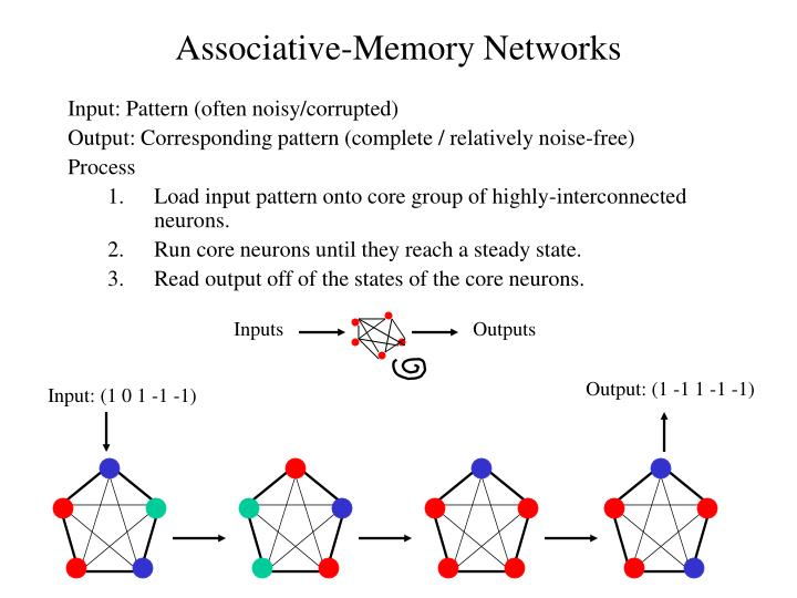
Inputs. Outputs. Associative-Memory Networks. Input: Pattern (often noisy/corrupted) Output: Corresponding pattern (complete / relatively noise-free) Process Load input pattern onto core group of highly-interconnected neurons. Run core neurons until they reach a steady state.

E N D
Inputs Outputs Associative-Memory Networks Input: Pattern (often noisy/corrupted) Output: Corresponding pattern (complete / relatively noise-free) Process • Load input pattern onto core group of highly-interconnected neurons. • Run core neurons until they reach a steady state. • Read output off of the states of the core neurons. Output: (1 -1 1 -1 -1) Input: (1 0 1 -1 -1)
Associative Network Types 1. Auto-associative: X = Y *Recognize noisy versions of a pattern 2. Hetero-associative Bidirectional: X <> Y BAM = Bidirectional Associative Memory *Iterative correction of input and output
Associative Network Types (2) 3. Hetero-associative Input Correcting: X <> Y *Input clique is auto-associative => repairs input patterns 4. Hetero-associative Output Correcting: X <> Y *Output clique is auto-associative => repairs output patterns
Hebb’s Rule Connection Weights ~ Correlations ``When one cell repeatedly assists in firing another, the axon of the first cell develops synaptic knobs (or enlarges them if they already exist) in contact with the soma of the second cell.” (Hebb, 1949) In an associative neural net, if we compare two pattern components (e.g. pixels) within many patterns and find that they are frequently in: a) the same state, then the arc weight between their NN nodes should be positive b) different states, then ” ” ” ” negative Matrix Memory: The weights must store the average correlations between all pattern components across all patterns. A net presented with a partial pattern can then use the correlations to recreate the entire pattern.
Correlated Field Components • Each component is a small portion of the pattern field (e.g. a pixel). • In the associative neural network, each node represents one field component. • For every pair of components, their values are compared in each of several patterns. • Set weight on arc between the NN nodes for the 2 components ~ avg correlation. a a ?? ?? b b Avg Correlation wab a b
Quantifying Hebb’s Rule Compare two nodes to calc a weight change that reflects the state correlation: * When the two components are the same (different), increase (decrease) the weight Auto-Association: i = input component o = output component Hetero-Association: Ideally, the weights will record the average correlations across all patterns: Auto: Hetero: Hebbian Principle: If all the input patterns are known prior to retrieval time, then init weights as: Auto: Hetero: Weights = Average Correlations
In Pattern 1: x1,1..x1,n Out P1: y1,1.. y1,j……y1,n In Pattern 2: x2,1..x2,n Out P2: y2,1.. y2,j……y2,n : : In Pattern p: x1,1..x1,n Out P3: yp,1.. yp,j ……yp,n Matrix Representation Let X = matrix of input patterns, where each ROW is a pattern. So xk,i = the ith bit of the kth pattern. Let Y = matrix of output patterns, where each ROW is a pattern. So yk,j = the jth bit of the kth pattern. Then, avg correlation between input bit i and output bit j across all patterns is: 1/P (x1,iy1,j + x2,iy2,j + … + xp,iyp,j) = wi,j To calculate all weights: Hetero Assoc: W = XTY Auto Assoc: W = XTX XT Y X Dot product P1 P2 Pp X1,i X2,i Xp,i ..
1 2 1 2 3 4 3 4 1 2 4 3 Auto-Associative Memory 1. Auto-Associative Patterns to Remember 3. Retrieval Comp/Node value legend: dark (blue) with x => +1 dark (red) w/o x => -1 light (green) => 0 1 2 3 4 2. Distributed Storage of All Patterns: 1 2 3 4 -1 1 1 2 3 4 • 1 node per pattern unit • Fully connected: clique • Weights = avg correlations across • all patterns of the corresponding units 1 2 3 4
1 1 a 2 b 3 Hetero-Associative Memory 1. Hetero-Associative Patterns (Pairs) to Remember 3. Retrieval a 2 b 3 2. Distributed Storage of All Patterns: 1 -1 a 2 1 b 3 • 1 node per pattern unit for X & Y • Full inter-layer connection • Weights = avg correlations across • all patterns of the corresponding units
Hopfield Networks • Auto-Association Network • Fully-connected (clique) with symmetric weights • State of node = f(inputs) • Weight values based on Hebbian principle • Performance: Must iterate a bit to converge on a pattern, but generally much less computation than in back-propagation networks. Input Output (after many iterations) Discrete node update rule: Input value
1 2 3 4 1/3 1 2 [-] 1/3 -1/3 -1/3 p1 p2 p3 Avg [+] 1/3 4 3 W12 1 1 -1 1/3 -1 W13 1 -1 -1 -1/3 W14 -1 1 1 1/3 W23 1 -1 1 1/3 W24 -1 1 -1 -1/3 +1 0 -1 W34 -1 -1 -1 -1 Hopfield Network Example 1. Patterns to Remember 3. Build Network p1 p3 p2 1 2 1 2 3 4 3 4 2. Hebbian Weight Init: Avg Correlations across 3 patterns 4. Enter Test Pattern 1/3 1 2 1/3 -1/3 -1/3 3 4 1/3 -1
Hopfield Network Example (2) 5. Synchronous Iteration (update all nodes at once) Inputs From discrete output rule: sign(sum) Node 1 2 3 4Output 1 1 00 -1/3 1 2 1/3 0 0 1/3 1 3 -1/3 0 0 1 1 4 1/3 0 0 -1 -1 Values from Input Layer 1/3 p1 1/3 = 1 2 -1/3 -1/3 1/3 3 4 -1 Stable State
Using Matrices Goal: Set weights such that an input vector Vi, yields itself when multiplied by the weights, W. X = V1,V2..Vp, where p = # input vectors (i.e., patterns) So Y=X, and the Hebbian weight calculation is: W = XTY = XTX 1 1 -1 1 1 1 -1 1 1 1 X = 1 1 -1 1 XT= 1 -1 1 -1 1 1 -1 -1 1 -1 3 1 -1 1 Common index = pattern #, so XTX = 1 3 1 -1 this is correlation sum. -1 1 3 -3 1 -1 -3 3 w2,4 = w4,2 = xT2,1x1,4 + xT2,2x2,4 + xT2,3x3,4
Matrices (2) • The upper and lower triangles of the product matrix represents the 6 weights wi,j = wj,i • Scale the weights by dividing by p (i.e., averaging) . Picton (ANN book) subtracts p from each. Either method is fine, as long we apply the appropriate thresholds to the output values. • This produces the same weights as in the non-matrix description. • Testing with input = ( 1 0 0 -1) 3 1 -1 1 (1 0 0 -1) 1 3 1 -1 = (2 2 2 -2) -1 1 3 -3 1 -1 -3 3 Scaling* by p = 3 and using 0 as a threshold gives: (2/3 2/3 2/3 -2/3) => (1 1 1 -1) *For illustrative purposes, it’s easier to scale by p at the end instead of scaling the entire weight matrix, W, prior to testing.
1/3 1 2 1/3 -1/3 -1/3 3 4 1/3 Spurious Outputs -1 • Input pattern is stable, • but not one of the • original patterns. • Attractors in node-state • space can be whole • patterns, parts of • patterns, or other • combinations. Hopfield Network Example (3) 4b. Enter Another Test Pattern 5b. Synchronous Iteration Inputs Node 1 2 3 4Output 1 1 1/30 0 1 2 1/3 1 0 0 1 3 -1/3 1/3 0 0 0 4 1/3 -1/3 0 0 0
1/3 1/3 -1/3 -1/3 1/3 -1 1/3 1/3 1/3 1/3 -1/3 -1/3 -1/3 -1/3 1/3 1/3 -1 -1 Hopfield Network Example (4) 4c. Enter Another Test Pattern 1 2 Asynchronous Updating is central to Hopfield’s (1982) original model. 3 4 5c. Asynchronous Iteration (One randomly-chosen node at a time) Update 3 Update 4 Update 2 Stable & Spurious 1/3 1/3 -1/3 -1/3 1/3 -1
Hopfield Network Example (5) 4d. Enter Another Test Pattern 1/3 1 2 1/3 -1/3 -1/3 3 4 1/3 -1 5d. Asynchronous Iteration Update 3 Update 4 Update 2 Stable Pattern p3 1/3 1/3 1/3 1/3 1/3 1/3 -1/3 -1/3 -1/3 -1/3 -1/3 -1/3 1/3 1/3 1/3 -1 -1 -1
1/3 1/3 1/3 1/3 -1/3 -1/3 -1/3 -1/3 1/3 1/3 -1 -1 Hopfield Network Example (6) 4e. Enter Same Test Pattern 1/3 1 2 1/3 -1/3 -1/3 3 4 1/3 -1 5e. Asynchronous Iteration (but in different order) Update 2 Update 3 or 4 (No change) Stable & Spurious
Associative Retrieval = Search p3 p1 p2 • Back-propagation: • Search in space of weight vectors to minimize output error • Associative Memory Retrieval: • Search in space of node values to minimize conflicts between a) node-value pairs • and average correlations (weights), and b) node values and their initial values. • Input patterns are local (sometimes global) minima, but many • spurious patterns are also minima. • High dependence upon initial pattern and update sequence (if asynchronous)
Energy Function Basic Idea: Energy of the associative memory should be low when pairs of node values mirror the average correlations (i.e. weights) on the arcs that connect the node pair, and when current node values equal their initial values (from the test pattern). When pairs match correlations, wkjxjxk > 0 When current values match input values, Ikxk > 0 Gradient Descent A little math shows that asynchronous updates using the discrete rule: yield a gradient descent search along the energy landscape for the E defined above.
Storage Capacity of Hopfield Networks Capacity = Relationship between # patterns that can be stored & retrieved without error to the size of the network. Capacity = # patterns / # nodes or # patterns / # weights • If we use the following definition of 100% correct retrieval: When any of the stored patterns is entered completely (no noise), then that same pattern is returned by the network; i.e. The pattern is a stable attractor. • A detailed proof shows that a Hopfield network of N nodes can achieve 100% correct retrieval on P patterns if: P < N/(4*ln(N)) NMax P 10 1 100 5 1000 36 10000 271 1011 109 In general, as more patterns are added to a network, the avg correlations will be less likely to match the correlations in any particular pattern. Hence, the likelihood of retrieval error will increase. => The key to perfect recall is selective ignorance!!
Stochastic Hopfield Networks Node state is stochastically determined by sum of inputs: Node fires with probability: For these networks, effective retrieval is obtained when P < 0.138N, which is an improvement over standard Hopfield nets. Boltzmann Machines: Similar to Hopfield nets but with hidden layers. State changes occur either: a. Deterministically when b. Stochastically with probability = Where t is a decreasing temperature variable and is the expected change in energy if the change is made. The non-determinism allows the system to ”jiggle” out of local minima.
Hopfield Nets in the Brain?? • The cerebral cortex is full of recurrent connections, and there is solid evidence for Hebbian synapse modification there. Hence, the cerebrum is believed to function as an associative memory. • Flip-flop figures indicate distributed hopfield-type coding, since we cannot hold both perceptions simultaneously (binding problem)
H E G F D A B C Closer(C,D) Closer(H,G) Closer(G,H) Excitatory Inhibitory Showing(G) Hidden(G) Closer(A,B) Convex(A) Convex(G) The Necker Cube Which face is closer to the viewer? BCGF or ADHE? Only one side of the (neural) network can be active at a time. Steven Pinker (1997) “How the Mind Works”, pg. 107.
Things to Remember • Auto-Associative -vs- Hetero-associative • Wide variety of net topologies • All use Hebbian Learning => weights ~ avg correlations • One-shot -vs- Iterative Retrieval • Iterative gives much better error correction. • Asynchronous -vs- Synchronous state updates • Synchronous updates can easily lead to oscillation • Asynchronous updates can quickly find a local optima (attractor) • Update order can determine attractor that is reached. • Pattern Retrieval = Search in node-state space. • Spurious patterns are hard to avoid, since many are attractors also. • Stochasticity helps jiggle out of local minima. • Memory load increase => recall error increase. • Associative -vs- Feed-Forward Nets • Assoc: Many - 1 mapping Feed-Forward: many-many mapping • Backprop is resource-intensive, while Hopfield iterative update is O(n) • Gradient-Descent on an Error -vs- Energy Landscape: • Backprop => arc-weight space Hopfield => node-state space