Download
1 / 22
220 likes | 331 Views
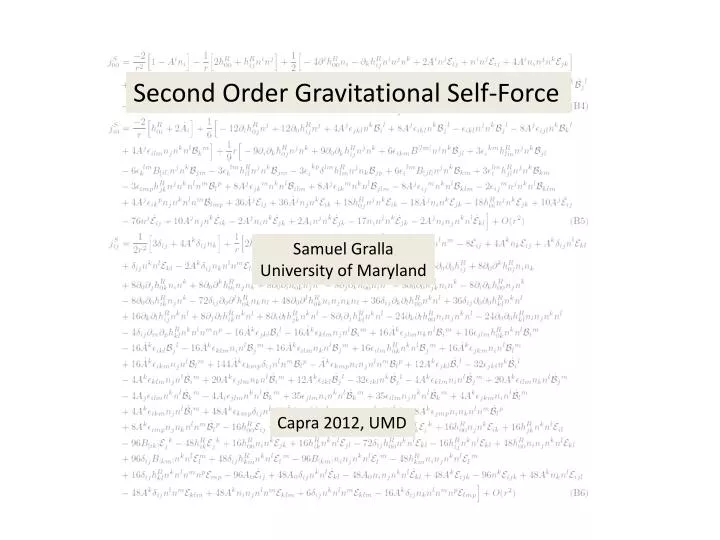
Second Order Gravitational Self-Force. Samuel Gralla University of Maryland. Capra 2012, UMD. Motion of Small Bodies. Consider a body that is small compared to the scale of variation of the external universe. Imagine expanding in the size/mass M of the body.

E N D
Second Order Gravitational Self-Force Samuel Gralla University of Maryland Capra 2012, UMD
Motion of Small Bodies Consider a body that is small compared to the scale of variation of the external universe. Imagine expanding in the size/mass M of the body. At least to some finite order in M, one would expect to be able to describe the body as following a worldline in a background spacetime. What is the acceleration of the worldline? M^0: zero (geodesic motion). ~100 years old; many derivations; no controversy. M^1: MiSaTaQuWa force. ~15 years old; several derivations; some controversy. M^2: no standard expression; much controversy M^n: ??? “second order gravitational self-force”
Difficulties with Point Particles Point particle sources don’t make sense in GR (Geroch and Traschen 1987) no mathematical meaning Full GR: We could try to fix things by taking M small, M^1: meaningful Now the equation is linear and makes sense. What about going to order M^2? okay okay M^2: not a distribution no mathematical meaning Involves products of the distribution g(1); Off Z, diverges as (x-Z)-4 not locally integrable
What equation gives the metric of a small body to O(M^2)??? We must return to a finite size body and consider a limit of small size/mass M. One way to do this is with the formalism of SEG & Wald 2008. To motivate our assumptions, consider approximating the Schwarzschild deSitter metric by using a parameter lambda, As λ0 we recover deSitter (the “background metric”), The body has shrunk to zero size and disappeared altogether.
1-param family: But there is another interesting limit. Introduce “scaled coordinates” and the family becomes, and you get Also introduce a new, scaled metric Now the limit as λ0 yields the “body metric” of Schwarzschild, This procedure has “zoomed in” on the body, because the coordinates scale at the same rate as the body.
We assume a one-parameter-family g(λ) where ordinary and scaled limits of this sort exist and are smoothly related to each other in a certain sense. The main output is a form of the perturbative metric, These coordinates have the background worldline of the particle (the place where it “disappeared to”) at r=0. anm are functions of time and angles The n^th order perturbation diverges as 1/r^n near the background worldline (Notice how this behavior was present in the example family, )
Einstein’s equation The perturbed Einstein equations… New notation: g: background (smooth) h: first perutrbation (1/r) j: second perturbation (1/r^2) …together with the assumed (singular) metric form contain the complete information about the metric perturbations. Okay, great. How do you find h and j in practice? In SEG&Wald we proved that, at first order, the above description is equivalent to the linearized Einstein equation sourced by a point paticle. (This derives the point particle description from extended bodies! See also Pound’s work.) But what do we do at second order, which doesn’t play nice with point particles?
Answer: Effective Source Method! Barack and Golbourn and Detweiler and Vega introduced a technique for determining the field of a point particle by considering smooth sources. We can recast their method in our language without ever mentioning point particles. Things then generalize to second order. (The only new wrinkle at first order is the gauge freedom; previous effective source work has considered Lorenz gauge only.)
Effective source at first order in our approach: We know that and h ~ 1/r near r=0 At some level we have a “singular boundary condition”. How to remove it? Solve analytically for h in series in r. Find the general solution in a particular gauge. (explicit expressions given) The solution contains free functions. But note by inspection that we may isolate off a “singular piece” hS such that • hS has no free functions (depends only on M and background curvature) • hP – hS is C^2 at r=0 (or some desired smoothness) Pick this hS and call it the “singular field”.
Our choice of “singular field”: (expressed in a local inertial coordinate system of the background metric about the background worldline) The claim is that the general solution has h-hS sufficiently regular when h is expressed in a particular gauge (“P gauge”). But now consider any smoothly related gauge (“P-smooth gauges”), (Xi smooth) It is of course still true that h-hS is sufficiently regular.
So we have a “singular field” and a corresponding class of gauges such that h-hS is always sufficiently regular. Choose an arbitrary extension of hS to the entire manifold and define (hats denote extended quantities) Then Einstein’s equation, becomes Can drop! The right-hand-side is the “effective source” and is C^0. No more “singular boundary condition”. Numerical integrators happy. Pick initial/boundary conditions representing the physics of interest and pick any gauge condition (such as Lorenz on hR) such that hR is C^2. Then h = hR+hS is the physical metric perturbation expressed in a P-smooth gauge.
Effective source at second order: We have and j ~ 1/r^2 near r=0 To remove the “singular boundary condition” find the general solution in a particular gauge in series in r. (explicit expressions given) New subtlety: a smooth gauge transformation changes j by a singular amount! singular also singular! (xi, Xi smooth) We must include the second term in the singular field jS. We need to determine xi!
Determining xi We gave a prescription for computing h in a P-smooth gauge, (Xi smooth) Now that we know h we need to “invert” this equation and solve for xi. Recall that hP contains free functions. It turns out these are determined uniquely by h and xi. Then we have an equation just for xi. After some work we find a complicated expression for the general solution, which depends on 1) Background curvature 2) The regular field 3) A choice of “initial data” for the value and derivative of xi on the background worldline. (A and B obey transport equations) (A and B are value and derivative of xi on the background worldline)
Choose the second-order singular field to be Choose an arbitrary extension of jS to the entire manifold and define (hats denote extended quantities) Then Einstein’s equation, becomes Can drop! The right-hand-side is the “effective source” and is bounded. No more “singular boundary condition”. Numerical integrators happy. Pick initial/boundary conditions representing the physics of interest and pick any gauge condition (such as Lorenz on jR) such that jR is C^1. Then j = jR+jS is the physical metric perturbation expressed in a P-smooth gauge.
This provides a prescription for computing the metric of a small body through second order in its size/mass. You can do a lot with just this: fluxes, snapshot waveforms, etc. But what about the motion? Actually, with all this hard work done, it’s trivial. The secret is that we chose this P gauge to be “mass centered”: If you take the near-zone limit of the P-gauge metric perturbation, then the near-zone metric is just the ordinary Schwarzschild metric in isotropic coordinates. So, we say that the perturbed position of the particle vanishes in P gauge. But we worked in P-smooth gauges. What is the description there? Well, how does a point on the manifold “change” under a gauge transformation… New perturbed position:
So, we need to find the gauge vectors. Or do we? Here’s a trick: Let where this equation holds only in the P gauge. In a P smooth gauge we have Since the background motion is geodesic, vanishing perturbed motion means that the motion is geodesic in . This is an invariant statement and holds in any gauge! The motion is geodesic in the BG fields. This can be simply related to the regular fields that arise in practice, completing the prescription for determining the metric and motion. Recall jBG hBG
Second order Motion • “self-force”
The Prescription Choose a vacuum background spacetime and geodesic. Find a coordinate transformation between your favorite global coordinate system and my favorite local coordinate system (“RWZ coordinates”). Compute hS from the RWZ formula I give, choose an extension and compute the effective source, and solve for hR in some convenient gauge. Integrate some transport equations along the worldline to determine A and B, choosing trivial initial data. (A is the first-order motion.) Compute jS from the RWZ formula I give (involving also hR,A,B), choose an extension and compute the second-order effective source, and solve for jR a a convenient gauge. Integrate some more transport equations to get the second perturbed motion in your gauge.
What I have done… Given a prescription for computing the second order metric and motion perturbation of a small body. Good for local-in-time observables. What I haven’t done… Told you how to compute a long-term inspiral waveform. However, one should be able to apply adiabatic approaches (Mino; Hinderer and Flanagan) or self-consistent approaches, provided the role of gauge can be understood. What I would like to do… (or see others do!) Understand the role of gauge in adiabatic and self-consistent approaches.