Download
1 / 16
180 likes | 438 Views
Flipping an unfair coin three times. Consider the unfair coin with P(H) = 1/3 and P(T) = 2/3. If we flip this coin three times, the sample space S is the following set of ordered triples: S = {HHH, HHT, HTH, THH, TTH, THT, HTT, TTT}.

E N D
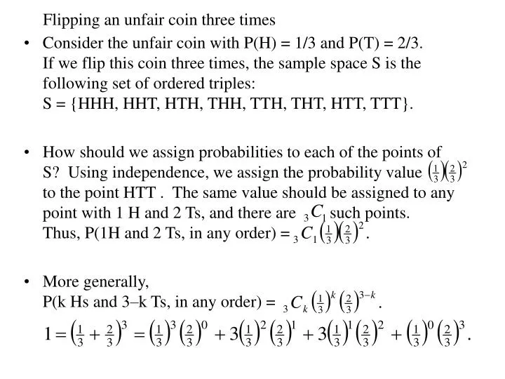
Flipping an unfair coin three times • Consider the unfair coin with P(H) = 1/3 and P(T) = 2/3. If we flip this coin three times, the sample space S is the following set of ordered triples: S = {HHH, HHT, HTH, THH, TTH, THT, HTT, TTT}. • How should we assign probabilities to each of the points of S? Using independence, we assign the probability value to the point HTT . The same value should be assigned to any point with 1 H and 2 Ts, and there are such points. Thus, P(1H and 2 Ts, in any order) = • More generally, P(k Hs and 3–k Ts, in any order) = • , in any order) =
Bernoulli trials • If we have a two outcome experiment that can be repeated in such a way that the outcome of an experiment does not affect the outcome of subsequent experiments, we call such an experiment a Bernoulli trial or a Bernoulli random variable. • We call the two outcomes of a Bernoulli trial “success” and “failure”. We suppose that the probability of “success” is p and the probability of “failure” is q, where p and q are positive and p + q = 1. • If n Bernoulli trials are carried out, then probabilities can be assigned in the fashion previously used for the unfair coin. This results in: P(k “successes” and n – k “failures”) =
Binomial random variable • The random variable X whose probability mass function is given by is said to be a binomial random variable with parameters n and p. • A binomial random variable gives the number of “successes” that occur when n independent trials, each of which result in a “success” with probability p, are performed. • Example. Let X be the number of girls born to a family with 5 children. X is a binomial r. v. with n = 5, p = 0.5. • Theorem. For a binomial r. v. X with parameters n and p,
Expected value for a binomial random variable: parameters n, p • E[X] = • The last summation equals 1, by the binomial theorem. Make sure you can justify all the steps shown above.
The maximum value of p(i) for a binomial r.v. • Let [t] denote the greatest integer less than or equal t. • Theorem. For a binomial random variable with parameters n and p, 0 < p < 1, the maximum value of the probability mass function p(i) occurs when • Example. Let n = 10, p = 0.5. Then the maximum of the probability mass function occurs at [11(0.5)] = 5. • Example. Let n = 11, p = 0.5. Then the maximum of the probability mass function occurs at [12(0.5)] = 6. By symmetry, the maximum also occurs at 11 – 6 = 5.
Error detection using a parity bit • ASCII code uses 7 bits and 1 parity bit. If an odd number of bits are flipped in transmission, the parity will be wrong and the error will be detected. If an even number of bits are flipped, the error will not be detected, however. Assume the probability of an error in transmission is 0.01 both for a 1 changing to 0 and for 0 changing to 1. Further assume that the probability for an error is the same regardless of the location of the error. • We let a “success” be flipping a bit and “failure” be flipping no bit. The parity checking situation is modeled as 8 Bernoulli trials. We have P(exactly one error) = P(exactly two errors) = which is quite small and the probabilities of four, six and eight errors are even smaller. We conclude that the probability of an error going undetected by the parity method is small.
Poisson random variable • The random variable X whose probability mass function is given by is said to be a Poisson random variable with parameter , and • A Poisson r. v. may be used as an approximation for a binomial r. v. with parameters (n, p) provided n is large and p is small enough that np has a moderate size (that is, np = for some constant ). • The Poisson approximation for a binomial is generally good if p < 0.1 and np 10. If np > 10, use the normal approximation in Chapter 7 of the textbook. • Example. The number of misprints on a page in a book is Poisson.
Example of Poisson Random Variable • Problem. Suppose that, on average, in every three pages of a book there is one typographical error. If the number of typographical errors on a single page is approximately a Poisson random variable, what is the probability of at least one error on a specific page of the book? Solution. Let X be the number of errors on the page we are interested in. Then X is Poisson with E(X) = 1/3 = , and Therefore,
Poisson Processes • Suppose that in the interval of time [0, t], we have a number of random events N(t) occurring. We note that for each t, N(t) is is a discrete r. v. with values in the nonnegative integers. We make the following assumptions for a Poisson process: • Stationarity: probability of n events in a time interval depends only on the length of the interval • Independent Increments: the number of events in nonoverlapping intervals are independent • Orderliness:
Theorem on existence of Poisson Process • Suppose that stationarity, independent increments, and orderliness hold, and N(0) = 0, and for all t > 0, then there exists a positive number such that That is, for all t > 0, N(t) is a Poisson r. v. with parameter Hence, E[N(t)] = and therefore, = E[N(1)]. • We say that the process described in the theorem is a Poisson process with rate . • For a Poisson process, suppose = 3. Evaluate
Probability that a car passes your house • Suppose that you check the traffic on the street in front of your house every day after lunch. Suppose further you find that about five vehicles pass by each hour. • Tomorrow after lunch you sit on a chair in front of your house at 1pm. What is the probability that at least one vehicle passes in the next 15 minutes? • Solution. Use a Poisson process with λ = 5 and t in hours. Therefore, the probability that at least one vehicle passes is 1– 0.2865 = 0.7135.
Fishing example • A fisherman catches fish at a Poisson rate of 2 per hour. Yesterday, he started fishing at 10 am and caught 1 fish by 10:30, and a total of 3 by noon. What is the probability that he can do this again tomorrow? Let the fishing tomorrow start at t = 0. • Make sure you can justify these steps.
Geometric random variable • The random variable X whose probability mass function is given by is said to be a geometric random variable with parameter p. • Such a random variable represents the trial number of the first success when each trial is independently a success with probability p. Its mean and variance are given by • Example. Draw a ball, with replacement, from an urn containing N white and M black balls. The number of draws required until a black ball is selected is a geometric random variable. What is p in this case?
Memoryless property of a geometric random variable • A discrete random variable X with values {1, 2, 3, … } is called memoryless in case, for all positive integers m and n, • Theorem. A geometric random variable is memoryless. Proof: • Interpretation of theorem: In successive independent Bernoulli trials, the probability that the next n outcomes are all failures does not change if we are given that the previous m successive outcomes were all failures.
Negative binomial random variable • The random variable X whose probability mass function is given by is said to be a negative binomial random variable with parameters r and p. • Such a random variable represents the trial number of the rth success when each trial is independently a success with probability p. Its mean and variance are given by • Example. Let X be the number of times one must throw a die until the outcome 1 has occurred 4 times. Then X is a negative binomial random variable with parameters r = 4 and p = 1/6.
Hypergeometric random variable • The random variable X whose probability mass function is given by is said to be a hypergeometric random variable with parameters n, N, and m. Note: n min(m, N – m). • Such a random variable represents the number of white balls selected when n balls are randomly chosen (without replacement) from an urn that contains N balls, of which m are white. With p = m/N, its mean and variance are • Problem. Suppose N = 10, n = 4, and m = 5. Let X be the number of white balls. What is P(X = 4)?