Download
1 / 94
960 likes | 1.19k Views
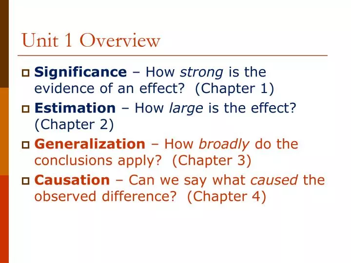
Unit 1 Overview. Significance – How strong is the evidence of an effect? (Chapter 1 ) Estimation – How large is the effect? (Chapter 2 ) Generalization – How broadly do the conclusions apply? (Chapter 3 ) Causation – Can we say what caused the observed difference? (Chapter 4).

E N D
Unit 1 Overview • Significance – How strong is the evidence of an effect? (Chapter 1) • Estimation – How large is the effect? (Chapter 2) • Generalization – How broadly do the conclusions apply? (Chapter 3) • Causation – Can we say what caused the observed difference? (Chapter 4)
Section 1.1: Introduction to Chance Models • Organ Donation Study • 78.6% in neutral group agreed • 41.8% in the opt-in group agreed • The researchers found these results to be statistically significant. • This means that if the recruitment method made no difference in the proportion that would agree, results as different as we found would be unlikely to arise by random chance.
Dolphin Communication • Can dolphins communicate abstract ideas? • In an experiment done in the 1960s, Doris was instructed which of two buttons to push. She then had to communicate this to Buzz (who could not see Doris). If he picked the correct button, both dolphins would get a reward. • What are the observational units and variables in this study?
Dolphin Communication • In one set of trials, Buzz chose the correct button 15 out of 16 times. • Based on these results, do you think Buzz knew which button to push or is he just guessing? • How might we justify an answer? • How might we model this situation?
Modeling Buzz and Doris • Flip Coins • One Proportion Applet
Three S Strategy • Statistic: Compute the statistic from the observed data. • Simulate: Identify a model that represents a chance explanation. Repeatedly simulate values of the statistic that could have happened when the chance model is true and form a distribution. • Strength of evidence: Consider whether the value of the observed statistic is unlikely to occur when the chance model is true.
Buzz and Doris Redo • Instead of a canvas curtain, Dr. Bastian constructed a wooden barrier between Buzz and Doris. • When tested, Buzz pushed the correct button only 16 out of 28 times. • Are these results statistically significant? • Let’s go to the applet to check this out.
Exploration 1.1: Can Dogs Understand Human Cues? (pg. 1-12) • Dogs were positioned 2.5 m from experimenter. • On each side of the experimenter were two cups. • The experimenter would perform some human cue (pointing, bowing or looking) towards one of the cups. (Non-human cues were also done.) • We will look at Harley’s results.
Section 1.2: Measuring Strength of Evidence • In the previous section we preformed tests of significance. • In this section we will make things slightly more complicated, formalize the process, and define new terminology.
We could take a look at Rock-Paper-Scissors-Lizard-Spock • Scissors cut paper • Paper covers rock • Rock crushes lizard • Lizard poisons Spock • Spock smashes scissors • Scissors decapitate lizard • Lizard eats paper • Paper disproves Spock • Spock vaporizes rock • (and as it always has) Rock crushes scissors RPS
Rock-Paper-Scissors • Rock smashes scissors • Paper covers rock • Scissors cut paper • Are these choices used in equal proportions (1/3 each)? • One study suggests that scissors are chosen less than 1/3 of the time.
Rock-Paper-Scissors • Suppose we are going to test this with 12 players each playing once against a computer. • What are the observational units? • What is the variable? • Even though there are three outcomes, we are focusing on whether the player chooses scissors or not. This is called a binary variable since we are focusing on 2 outcomes (not both necessarily equally likely).
Terminology: Hypotheses • When conducting a test of significance, one of the first things we do is give the null and alternative hypotheses. • The null hypothesis is the chance explanation. • Typically the alternative hypothesis is what the researchers think is true.
Hypotheses from Buzz and Doris • Null Hypothesis: Buzz will randomly pick a button. (He chooses the correct button 50% of the time, in the long run.) • Alternative Hypothesis: Buzz understands what Doris is communicating to him. (He chooses the correct button more than 50% of the time, in the long run.) These hypotheses represent the parameter (long run behavior) not the statistic (the observed results).
Hypotheses for R-P-S in words • Null Hypothesis: People playing Rock-Paper-Scissors will equally choose between the three options. (In particular, they will choose scissors one-third of the time, in the long run.) • Alternative Hypothesis: People playing Rock-Paper-Scissors will choose scissors less than one-third of the time, in the long run. Note the differences (and similarities) between these hypotheses and those for Buzz and Doris.
Hypotheses for R-P-S using symbols • H0: π = 1/3 • Ha: π< 1/3 where π is players’ true probability of throwing scissors
Setting up a Chance Model • Because the Buzz and Doris example had a 50% chance outcome, we could use a coin to model the outcome from one trial. What could we do in the case of Rock-Paper-Scissors?
Same Three S Strategy as Before • Statistic: Compute the statistic from the observed data. [In a class of 12 students, 2 picked scissors.This sample proportion can be described using the symbol (p-hat)]. • Simulate: Identify a model that represents a chance explanation. Repeatedly simulate values of the statistic that could have happened when the chance model is true and form a distribution. • Strength of evidence: Consider whether the value of the observed statistic is unlikely to occur when the chance model is true.
Applet • We will use the One Proportion Applet for our test. • This is the same applet we used last time except now we will change the proportion under the null hypothesis. • Let’s go to the applet and run the test. (Notice the use of symbols in the applet.)
P-value • The p-value is the proportion of the simulated statistics in the null distribution that are at least as extreme (in the direction of the alternative hypothesis) as the value of the statistic actually observed in the research study. • We should have seen something similar to this in the applet Proportion of samples: 938/5000 = 0.1876
What can we conclude? • Do we have strong evidence that less than 1/3 of the time scissors gets thrown? • How small of a p-value would you say gives strong evidence? • Remember the smaller the p-value, the stronger the evidence against the null.
Guidelines for evaluating strength of evidence from p-values • p-value >0.10, not much evidence against null hypothesis • 0.05 < p-value <0.10, moderate evidence against the null hypothesis • 0.01 < p-value <0.05, strong evidence against the null hypothesis • p-value <0.01, very strong evidence against the null hypothesis
What can we conclude? • So we do not have strong evidence that fewer than 1/3 of the time scissors is thrown. • Does this mean we can conclude that 1/3 of the time scissors is thrown? • Is it plausible that 1/3 of the time scissors is thrown? • Are other values plausible? Which ones? • What could we do to have a better chance of getting strong evidence for our alternative hypothesis?
Summary • The null hypothesis (H0) is the chance explanation. (=) • The alternative hypothesis (Ha) is you are trying to show is true. (< or >) • A null distribution is the distribution of simulated statistics that represent the chance outcome. • The p-value is the proportion of the simulated statistics in the null distribution that are at least as extremeas the value of the observed statistic.
Summary • The smaller the p-value, the stronger the evidence against the null. • P-values less than 0.05 provide strong evidence against the null. • πis the population parameter • is the sample proportion
Exploration 1.2 (pg 1-25) • Can people tell the difference between bottled and tap water?
Alternative Measure of Strength of Evidence Section 1.3
Criminal Justice System vs. Significance Tests • Innocent until proven guilty. We assume a defendant is innocent and the prosecutionhas to collect evidence to try to prove the defendant is guilty. • Likewise, we assume our chance model (or null hypothesis) is true and we collect data and calculate a sample proportion. We then show how unlikely our proportion is if the chance model is true.
Criminal Justice System vs. Significance Tests • If the prosecution shows lots of evidence that goes against this assumption of innocence (DNA, witnesses, motive, contradictory story, etc.) then the jury might conclude that the innocence assumption is wrong. • If after we collect data and find that the likelihood (p-value) of such a proportion is so small that it would rarely occur by chance if the null hypothesis is true, then we conclude our chance model is wrong.
Review • In the water tasting exploration, you could have obtained a null distribution similar to the one shown here. (H0: π = 0.25, Ha: π < 0.25 and = 3/27 = 0.1111) • What does a single dot represent? • What does the whole distribution represent? • What is the p-value for this simulation? • What does this p-value mean?
More Review • The null hypothesis is the chance explanation. • Typically the alternative hypothesis is what the researchers think is true. • The p-valueis the proportion of outcomes in the null distribution that are at least as extreme as the value of the statistic actually observed in the study. • Small p-values are evidence against the null.
Strength of Evidence • P-values are one measure for the strength of evidence and they are, by far, the most frequently used. • P-values essentially are measures of how far the sample statistic is away from the parameter under the null hypothesis. • Another measure for this distance we will look at today is called the standardized statistic.
Heart Transplant Operations Example 1.3
Heart Transplants • The British Medical Journal (2004) reported that heart transplants at St. George’s Hospital in London had been suspended after a spike in the mortality rate • Of the last 10 heart transplants, 80% had resulted in deaths within 30 days • This mortality rate was over five times the national average. • The researchers used 15% as a reasonable value for comparison.
Heart Transplants • Does a heart transplant patient at St. George’s have a higher probability of dying than the national rate of 0.15? • Observational units • The last 10 heart transplantations • Variable • If the patient died or not • Parameter • The actual long-run probability of a death after a heart transplant operation at St. George’s
Heart Transplants • Null hypothesis: Death rate at St. George’s is the same as the national rate (0.15). • Alternative hypothesis: Death rate at St. George’s is higher than the national rate. • H0: = 0.15 Ha: > 0.15 • Our statistic is 8 out of 10 or 0.80
Heart Transplants Simulation • Null distribution of 1000 repetitions of drawing samples of 10 “patients” where the probability of death is equal to 0.15. What is the p-value?
Heart Transplants Strength of Evidence • Our p-value is 0, so we have very strong evidence against the null hypothesis. • Even with this strong evidence, it would be nice to have more data. • Researchers examined the previous 361 heart transplantations at St. George’s and found that 71 died within 30 days. • Our new statistic is 71/361 ≈ 0.197
Heart Transplants • Here is a null distribution and p-value based on the new statistic.
Heart Transplants • The p-value was about 0.007 • We still have very strong evidence against the null hypothesis, but not quite as strong as the first case • Another way to measure strength of evidence is to standardize the observed statistic
The Standardized Statistic • The standardized statistic is the number of standard deviations our sample statistic is above the mean of the null distribution. • For a single proportion, we will use the symbol z for standardized statistic.
The standardized statistic • Here are the standardized statistics for our two studies. • In the first, our observed statistic was 5.70 standard deviations above the mean. • In the second, our observed statistic was 2.47 standard deviations above the mean. • Both of these are very strong, but we have stronger evidence against the null in the first.
Guidelines for strength of evidence • If a standardized statistic is below -2 or above 2, we have strong evidence against the null.
Do People Use Facial Prototyping? Exploration 1.3
Impacting Strength of Evidence Section 1.4
Introduction • We’ve now looked at tests of significance and have seen how p-values and standardized statistics give information about the strength of evidence against the null hypothesis. • Today we’ll explore factors that affect strength of evidence.