Download
1 / 29
290 likes | 394 Views
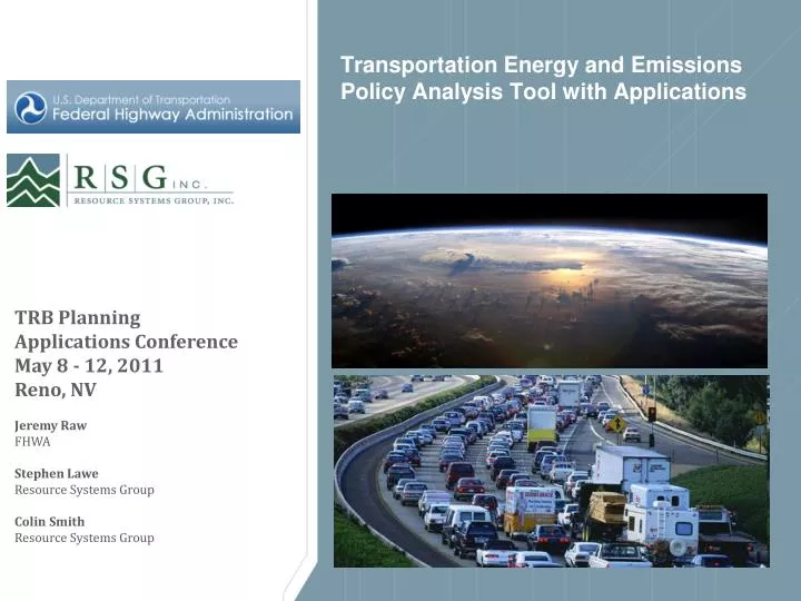
Transportation Energy and Emissions Policy Analysis Tool with Applications. TRB Planning Applications Conference May 8 - 12, 2011 Reno, NV Jeremy Raw FHWA Stephen Lawe Resource Systems Group Colin Smith Resource Systems Group. Presentation Overview. STEEP-AT:

E N D
Transportation Energy and EmissionsPolicy Analysis Tool with Applications TRB Planning Applications Conference May 8 - 12, 2011 Reno, NV Jeremy Raw FHWA Stephen Lawe Resource Systems Group Colin Smith Resource Systems Group
Presentation Overview • STEEP-AT: Strategic TransportationEnergyandEmissionsPolicyanalysis tool • Overview of STEEP-AT (Jeremy) • STEEP-AT application to Florida (Stephen)
FHWA Interest in Greenhouse Gas Planning • Guidelines and Procedures • Analysis Tools and Methods • Support for Policy Analysis • Mitigation Strategies • Policy Evaluation
Genesis of STEEP-AT • Based on theGreenSTEP model • GREENhouse gas Statewide Transportation Emissions Planning Model • Originally developed by the Oregon Department of Transportation (ODOT) Transportation Planning Analysis Unit (TPAU) • A modeling tool to assess the effects of policies and other factors on transportation sector GHG emissions • Built in the R statistical computing language • FHWA funded project to make available to other states www.r-project.org
FHWA Plans for STEEP-AT • Preliminary tool release is imminent (Summer 2011) • Free Software • Documentation • Case Studies (Oregon and Florida) • Testing with additional states • Project will be supported and potentially extended to other areas
Caveats for STEEP-AT • Not a “One Stop” Solution • Only Strategic Policy Analysis • Not for detailed emissions analysis (use MOVES) • Not for project level evaluation (use travel model + MOVES) • STEEP-AT operates on a county level and has been used for statewide policy testing
Model Sensitivities Land use and demographics Transportation supply • Population demographics (age structure) • Personal income • Relative amounts of development occurring in metropolitan, urban and rural areas • Metropolitan, other urban, and rural area densities • Urban form in metropolitan areas (proportion of population living in mixed use areas) • Amounts of metropolitan area transit service • Metropolitan freeway and arterial supplies Policies • Pricing: fuel, vehicle miles traveled (VMT), parking • Demand management – employer-based and individual marketing • Car-sharing • Effects of congestion on fuel economy • Effects of incident management on fuel economy • Vehicle operation and maintenance – eco-driving, low rolling resistance tires, speed limits • Carbon intensity of fuels, including the well to wheels emissions , and production of power to run electric vehicles. Vehicle fleet characteristics • Auto and light truck proportions by year • Average vehicle fuel economy by vehicle type and year • Vehicle age distribution by vehicle type • Electric vehicles (EVs), plug-in hybrid electric vehicles (PHEVs) • Light-weight vehicles such as bicycles, electric bicycles, electric scooters, etc.
STEEP-AT: Model Structure Recalculate household vehicle travel and adjust allocation to vehicles Generate synthetic households Aggregate characteristics by county, income group and development type Apply urban area land use and transportation system characteristics Model heavy vehicle VMT Model vehicle ownership types and ages Adjust MPG due to congestion Model initial estimates of household vehicle travel Calculate fuel consumption by type Model household vehicle types and allocate VMT to vehicles Calculate lifecycle CO2e emissions by fuel type Calculate household cost per vehicle mile
Data Inputs and Outputs Generate synthetic households • Inputs: • Population forecasts by county, age to 2040 • PUMS data • Household income forecasts • Outputs: • Synthetic population for the state • Household attributes include size, age of household members, and household income
Data Inputs and Outputs Generate synthetic households Apply urban area land use and transportation system characteristics Model vehicle ownership types and ages • Inputs: • NHTS data on vehicle ownership by household type • Outputs: • Vehicle ownership by household • Can be aggregated by household attributes, e.g. county, age, area type such as rural or metropolitan
Data Inputs and Outputs Generate synthetic households Apply urban area land use and transportation system characteristics Model vehicle ownership types and ages Model initial estimates of household vehicle travel • Inputs: • NHTS data on daily travel • Model sensitive to transportation supply data, land use (residential density), household attributes • Outputs: • Daily VMT by household
Data Inputs and Outputs Generate synthetic households Apply urban area land use and transportation system characteristics Model vehicle ownership types and ages Model initial estimates of household vehicle travel Model household vehicle types and allocate VMT to vehicles • Inputs: • NHTS data on vehicle ages • Outputs: • Vehicle age and VMT allocated to all vehicles
Data Inputs and Outputs Recalculate household vehicle travel and adjust allocation to vehicles Generate synthetic households Aggregate characteristics by county, income group and development type Apply urban area land use and transportation system characteristics Model heavy vehicle VMT Model vehicle ownership types and ages Adjust MPG due to congestion Model initial estimates of household vehicle travel Model household vehicle types and allocate VMT to vehicles Calculate household cost per vehicle mile
Data Inputs and Outputs Recalculate household vehicle travel and adjust allocation to vehicles Aggregate characteristics by county, income group and development type Model heavy vehicle VMT Adjust MPG due to congestion • Inputs: • Urban mobility report: speed vs ADT per lane • MOVES relationships between speed and fuel economy • Outputs: • Fuel used per day
Data Inputs and Outputs Recalculate household vehicle travel and adjust allocation to vehicles Aggregate characteristics by county, income group and development type Model heavy vehicle VMT Adjust MPG due to congestion Calculate fuel consumption by type • Inputs: • Fuel type proportions by year • Carbon intensity by fuel type • Outputs: • Emissions by fuel type and by vehicle type, by county Calculate lifecycle CO2e emissions by fuel type
STEEP-AT: Model Structure Recalculate household vehicle travel and adjust allocation to vehicles Generate synthetic households Aggregate characteristics by county, income group and development type Apply urban area land use and transportation system characteristics Model heavy vehicle VMT Model vehicle ownership types and ages Adjust MPG due to congestion Model initial estimates of household vehicle travel Calculate fuel consumption by type Model household vehicle types and allocate VMT to vehicles Calculate lifecycle CO2e emissions by fuel type Calculate household cost per vehicle mile
Policy testing in Oregon VMT Reduction GHG Reduction Marketing Pricing Roads Urban Fleet Tech • Objectives of Round 1 (completed) • Understand: • Magnitude of possible GHG emissions reductions • Change neededto reduce GHG emissions by 75% • Identify • Pathways to get Oregon to the reduction goal • Key factors/interactions for reducing GHG emissions • Scenarios to carry to next round of modeling • Round 2 is now underway • Several rounds of scenario development and modeling • Round 1: Broadly explore the territory to understand the possibilities, implications for meeting 2050 target. • Round 2: Narrow down potential scenarios, make adjustments, examine trajectories for GHG reduction: look at 2020 and 2035 as well as 2050. • Round 3: Further narrow/adjust scenarios. Evaluate and recommend leading candidate(s). • Modeled 144 combinations of levels of six policy groups: Urban Characteristics, Pricing, Marketing, Roads, Fleet Characteristics, Technology • Combination of highest levels reduces GHG by just over 70% • Technology (e.g. vehicle efficiency improvements) has the largest effect, then urban characteristics and pricing >60%
Application of STEEP-at in Florida
Data Inputs and Outputs 1. Model Transferability to Florida • Calculation based components, e.g. population synthesizer: updated input data (PUMS data) • Components estimated with national data, e.g. daily VMT model based on NHTS data, are transferable • Components based on state/regional data not transferable, re-estimated with local data, e.g. vehicle choice models 2. Computational Issues in FL vs. OR • R is an open source statistical analysis environment • Many calculations at household level: run times 2 hours per year per scenario vs. 40 minutes • Memory use: up to 6GB vs. <2GB, requires 64 bit OS to run on Windows *2005 is the model base year
Age Profiles in Oregon and Florida • In 2005 Oregon population was a little younger than Florida’s • 65 Plus group is 14% of population in Oregon, 18% in Florida • The gap is forecast to widen between now and 2040
Age Profiles in Oregon and Florida In 2040, the 65 Plus segment of the population is forecast to be 21% in Oregon, and 32% in Florida
Age in STEEP-AT Generate synthetic households Model initial estimates of household vehicle travel • Population synthesizer creates a population that has the correct age profile • Household income model assigns incomes based on age profile in the household Recalculate household vehicle travel and adjust allocation to vehicles • Models predict lower VMT for lower incomes and lower vehicle ownership • Plus 65 households more likely to have zero VMT, lower average VMT • Budget constraint models the effects of travel costs: lower income households affected more by price increases, e.g. higher gas prices Model vehicle ownership types and ages • Models include income variables (which are dependent on age) • Households with only plus 65s more likely to be zero vehicle or low vehicle ownership households Other policy responses • Workplace TDM: have to be in workforce • EV, PHEV: depends on daily VMT, plus 65s more likely to stay within charge range
More People = More Emissions 0 7,500 CO2eq Emissions in Tons / Day Cities > 100,000 people in 1990
Case Study: increased Electric Vehicle use • Electric plug in vehicles are now being introduced, with Federal, State and local incentives for consumers. • How much will CO2 be reduced if these vehicles gain market share? • Scenario: • 2040 • Typical electric autos range = 100 miles • Typical electric light trucks range = 200 miles • 40% of all autos and light trucks that drive up to average electric range are electric vehicles • GreenSTEP approach: • Electric vehicle power consumption converted into CO2 equivalents • Emissions rate per kWh power consumed reflect the overall average for all power consumed in Oregon, 1.114 pounds/kWh • It does not distinguish differences between power providers, but it is an end-user rate (includes power transmission loss effects) • Nissan Leaf • First US deliveries due in December 2010 • Battery powered electric car • Range 100 miles in city driving • Lithium ion battery pack, 24kWh capacity • Recharge time from empty: • 120V/15amp household outlet = 20 hours • 240V/30amp home charging dock = 8 hours • 500V commercial charging station = 30 min
Plug In Autos - Where Matters Cleanest States Dirtiest States Nuclear Power Plants Renewable Power Plants CO2 lbs/MWh scaled 3300 200 26
Knowledge of the Electric Grid Analysis uses the Florida Reliability Coordinating Council’s region
Impact of Accounting for Marginal Facilities • Ignoring electric sector misses ~ 4.7 billion pounds of GHG emissions in 2040 alone. • This is equivalent to not counting 400,000 gas-fired cars in the Florida fleet. • Analysis uses the Florida Reliability Coordinating Council’s region RSG uses the hour by hour plug-in demand matched against the region’s fluctuating marginal power plant mix. Oregon GreenSTEPassumes a system average for all hours of the year.