Download
1 / 29
290 likes | 304 Views
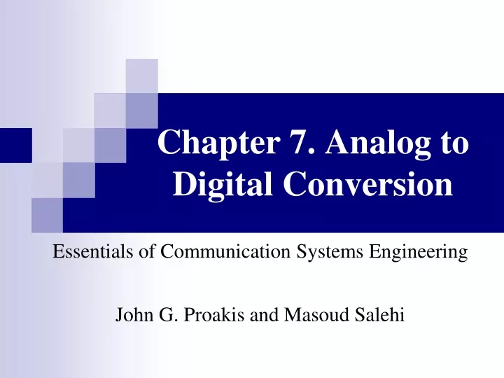
Chapter 7. Analog to Digital Conversion. Essentials of Communication Systems Engineering John G. Proakis and Masoud Salehi. Chapter 7. Analog to Digital Conversion. In order to convert an analog signal to a digital signal, i.e., a stream of bits, three operations must be completed.

E N D
Chapter 7. Analog to Digital Conversion Essentials of Communication Systems Engineering John G. Proakis and Masoud Salehi
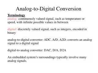
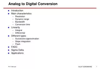
Chapter 7. Analog to Digital Conversion • In order to convert an analog signal to a digital signal, i.e., a stream of bits, • three operations must be completed. • First, the analog signal has to be sampled, so that we can obtain a discrete-time continuous-valued signal from the analog signal.This operation is called sampling. • Then the sampled values, which can take an infinite number of values are quantized, i.e., rounded to a finite number of values. This is called the quantization process. • After quantization, we have a discrete-time, discrete-amplitude signal. The third stage in analog-to-digital conversion is encoding. In encoding, a sequence of bits (ones and zeros) are assigned to different outputs of the quantizer. Since the possible outputs of the quantizer are finite, each sample of the signal can be represented by a finite number of bits. For instance, if the quantizer has 256 = 28 possible levels, they can be represented by 8 bits. Oh-Jin Kwon, EE dept., Sejong Univ., Seoul, Korea: http://dasan.sejong.ac.kr/~ojkwon/
7.1 Sampling of Signals and Signal Reconstruction from Samples 7.1.1 The Sampling Theorem Figure 7.1 Sampling of signals. Oh-Jin Kwon, EE dept., Sejong Univ., Seoul, Korea: http://dasan.sejong.ac.kr/~ojkwon/
The (Shannon’s) Sampling Theorem: • It basically states two facts: • If the signal x(t) is bandlimited to W, i.e., if X(f) 0 for |f| W, then it is sufficient to sample at intervals Ts = 1/(2W) recover the exact original signal from the samples. • We may recover the signal x(t) by lowpass filtering the samples with the cutoff frequency W. • Proof) Oh-Jin Kwon, EE dept., Sejong Univ., Seoul, Korea: http://dasan.sejong.ac.kr/~ojkwon/
Sampling Theorem • Now if Ts > 1/(2W), then the replicated spectrum of x(t)overlaps and reconstruction of the original signal is not possible. • This type of distortion, which results from undersampling, is known as aliasing error or aliasing distortion. • However, if Ts 1/(2W), no overlap occurs; and by employing an appropriate filter we can reconstruct the original signal. Figure 7.2 Frequency-domain representation of the sampled signal. Oh-Jin Kwon, EE dept., Sejong Univ., Seoul, Korea: http://dasan.sejong.ac.kr/~ojkwon/
Sampling Theorem • The sampling rate fs= 2W is the minimum sampling rate at which no aliasing occurs. • This sampling rate is known as the Nyquist sampling rate. • If sampling is done at the Nyquist rate, then the only choice for the reconstruction filter is an ideal lowpass filter and W' = W = 1/(2Ts). • In practical systems, sampling is done at a rate higher than the Nyquist rate. • This allows for the reconstruction filter to be realizable and easier to build. • In such cases, the distance between two adjacent replicated spectra in the frequency domain, i.e., (1/Ts - W) - W = fs- 2W, is known as the guard band. • Therefore, in systems with a guard band, we have fs = 2W + WG, where W is the bandwidth of the signal, WGis the guard band, and fsis the sampling frequency. Oh-Jin Kwon, EE dept., Sejong Univ., Seoul, Korea: http://dasan.sejong.ac.kr/~ojkwon/
7.1.2 (Analog) Pulse Modulation • Pulse Amplitude Modulation (PAM) • Sample and hold • Instantaneous sampling • Lengthening(T) • Pulse Duration/Width Modulation (PDM/PWM) • Samples of the message signal are used to vary the duration(width) of the individual pulses in the carrier • Pulse Position Modulation (PPM) • The position of a pulse relative to its unmodulated time of occurrence is varied in accordance with the message signal Oh-Jin Kwon, EE dept., Sejong Univ., Seoul, Korea: http://dasan.sejong.ac.kr/~ojkwon/
(Analog) Pulse Modulation : Demodulation은 역순으로 • PPM Pulse 높이 > 0 Oh-Jin Kwon, EE dept., Sejong Univ., Seoul, Korea: http://dasan.sejong.ac.kr/~ojkwon/ PDM(PWM)
7.2 QUANTIZATION • After sampling, we have a discrete-time signal, i.e., a signal with values at integer multiples of Ts. • The amplitudes of these signals are still continuous, however. • Transmission of real numbers requires an infinite number of bits, since generally the base 2 representation of real numbers has infinite length. • After sampling, we will use quantization, in which the amplitude becomes discrete as well. • As a result, after the quantization step, we will deal with a discrete-time, finite-amplitude signal, in which each sample is represented by a finite number of bits. Oh-Jin Kwon, EE dept., Sejong Univ., Seoul, Korea: http://dasan.sejong.ac.kr/~ojkwon/
7.2.1 Scalar Quantization • In scalar quantization • Each sample is quantized into one of a finite number of levels which is then encoded into a binary representation. • The quantization process is a rounding process; each sampled signal point is rounded to the "nearest" value from a finite set of possible quantization levels. • The set of real numbers R is partitioned into N disjoint subsets denoted by Rk, 1 k N(each called a quantization region). • Corresponding to each subset Rk,a representation point (or quantization level) is chosen, which usually belongs to Rk. • If the sampled signal at time i , xibelongs to Rk,then it is represented by , which is the quantized version of x. • Then, is represented by a binary sequence and transmitted. This latter step is called encoding. • Since there are N possibilities for the quantized levels, log2N bits are enough to encode these levels into binary sequences. • Therefore, the number of bits required to transmit each source output is R = log2 N bits. • The price that we have paid for representing (rounding) every sample that falls in the region Rkby a single point is the introduction of distortion. Oh-Jin Kwon, EE dept., Sejong Univ., Seoul, Korea: http://dasan.sejong.ac.kr/~ojkwon/
Scalar Quantization • Figure 7.3 shows an example of an 8-level quantization scheme. • In this scheme, the eight regions are defined as R1 = (-, a1), R2 = (a1, a2), , R8 = (a8, -). • The representation point (or quantized value) in each region is denoted by and is shown in the figure. • The quantization function Q is defined by Figure 7.3 Example of an 8-level quantization scheme. Oh-Jin Kwon, EE dept., Sejong Univ., Seoul, Korea: http://dasan.sejong.ac.kr/~ojkwon/
Scalar Quantization • Depending on the measure of distortion employed, we can define the average distortion resulting from quantization. • A popular measure of distortion, used widely in practice, is the squared error distortion defined as (x – )2. • In this expression x is the sampled signal value and is the quantized value, i.e., = Q (x). • If we are using the squared error distortion measure, then where = x - Q (x). • Since X is a random variable, so are and ; therefore, the average (mean squared error) distortion is given by • Mean squared distortion, or quantization noise as the measure of performance. • A more meaningful measure of performance is a normalized version of the quantization noise, and it is normalized with respect to the power of the original signal. Oh-Jin Kwon, EE dept., Sejong Univ., Seoul, Korea: http://dasan.sejong.ac.kr/~ojkwon/
Uniform Quantization • Uniform quantizers are the simplest examples of scalar quantizers. • In a uniform quantizer, the entire real line is partitioned into N regions. • All regions except R1and RNare of equal length, which is denoted by . • This means that for all 1 i N - 1, we have ai+l- ai= . • It is further assumed that the quantization levels are at a distance-of /2 from the boundaries a1, a2,..., aN-1 : Figure 7.3is an example of an 8-level uniform quantizer. • In a uniform quantizer, the mean squared error distortion is given by • Thus, D is a function of two design parameters, namely, a1and . • In order to design the optimal uniform quantizer, we have to differentiate D with respect to these variables and find the values that minimize D. • Minimization of distortion is generally a tedious task and is done mainly by numerical techniques. • Table 7.1 gives the optimal quantization level spacing for a zero-mean unit-variance Gaussian random variable : • The last column in the table gives the entropy after quantization. Oh-Jin Kwon, EE dept., Sejong Univ., Seoul, Korea: http://dasan.sejong.ac.kr/~ojkwon/
Uniform Quantization Oh-Jin Kwon, EE dept., Sejong Univ., Seoul, Korea: http://dasan.sejong.ac.kr/~ojkwon/
Nonuniform Quantization • If we relax the condition that the quantization regions (except for the first and the last one) be of equal length, then we are minimizing the distortion with less constraints • Therefore, the resulting quantizer will perform better than a uniform quantizer with the same number of levels. • Let us assume that we are interested in designing the optimal mean squared error quantizer with N levels of quantization with no other constraint on the regions. • The average distortion will be given by • There exists a total of 2N - 1 variables in this expression (a1, a2, . . . , aN-1)and and the minimization of D is to be done with respect to these variables. • Differentiating with respect to aiyields • This result simply means that, in an optimal quantizer, the boundaries of the quantization regions are the midpoints of the quantized values. • Because quantization is done on a minimum distance basis, each x value is quantized to the nearest (7.2.10) Oh-Jin Kwon, EE dept., Sejong Univ., Seoul, Korea: http://dasan.sejong.ac.kr/~ojkwon/
Nonuniform Quantization • To determine the quantized values , we differentiate Dwith respect to and define a0= -and aN = +. • Thus, we obtain • Equation (7.2.12) shows that in an optimal quantizer, the quantized value (or representation point) for a region should be chosen to be the centroid of that region. • Equations (7.2.10) and (7.2.12) give the necessary conditions for a scalar quantizer to be optimal; they are known as the Lloyd-Max conditions. • The criteria for optimal quantization (the Lloyd-Max conditions) can then be summarized as follows: 1. The boundaries of the quantization regions are the midpoints of the corresponding quantized values (nearest neighbor law). 2. The quantized values are the centroids of the quantization regions. (7.2.12) Oh-Jin Kwon, EE dept., Sejong Univ., Seoul, Korea: http://dasan.sejong.ac.kr/~ojkwon/
Nonuniform Quantization • Although these rules are very simple, they do not result in analytical solutions to the optimal quantizer design. • The usual method of designing the optimal quantizer is to start with a set of quantization regions and then, using the second criterion, to find the quantized values. • Then, we design new quantization regions for the new quantized values, and alternate between the two steps until the distortion does not change much from one step to the next. • Based on this method, we can design the optimal quantizer for various source statistics. • Table 7.2 shows the optimal nonuniform quantizers for various values of N for a zero-mean unit-variance Gaussian source. • If, instead of this source, a general Gaussian source with mean m and variance 2is used, then the values of ai and read from Table 7.2 are replaced with m + aiand m + , respectively, and the value of the distortion D will be replaced by 2D. Oh-Jin Kwon, EE dept., Sejong Univ., Seoul, Korea: http://dasan.sejong.ac.kr/~ojkwon/
Nonuniform Quantization Oh-Jin Kwon, EE dept., Sejong Univ., Seoul, Korea: http://dasan.sejong.ac.kr/~ojkwon/
7.4.1 Pulse Code Modulation (PCM) • Pulse code modulation is the simplest and oldest waveform coding scheme. • A pulse code modulator consists of three basic sections: a sampler, a quantizer and an encoder. • A functional block diagram of a PCM system is shown in Figure 7.7. • In PCM, we make the following assumptions: • The waveform (signal) is bandlimited with a maximum frequency of W. Therefore, it can be fully reconstructed from samples taken at a rate of fs= 2W or higher. • The signal is of finite amplitude. In other words, there exists a maximum amplitude xmax such that for all t , we have |x(t)| xmax. • The quantization is done with a large number of quantization levels N, which is a power of 2 (N = 2v). Figure 7.7 Block diagram of a PCM system. Oh-Jin Kwon, EE dept., Sejong Univ., Seoul, Korea: http://dasan.sejong.ac.kr/~ojkwon/
7.4.2 Differential Pulse Code Modulation (DPCM) • PCM system • After sampling the information signal, each sample is quantized independently using a scalar quantizer. • Previous sample values have no effect on the quantization of the new samples. • DPCM System • When a bandlimited random process is sampled at the Nyquist rate or faster, the sampled values are usually correlated random variables. • The exception is the case when the spectrum of the process is flat within its bandwidth. • The previous samples give some information about the next sample • This information can be employed to improve the performance of the PCM system. • If the previous sample values were small, and there is a high probability that the next sample value will be small as well, then it is not necessary to quantize a wide range of values to achieve a good performance. Oh-Jin Kwon, EE dept., Sejong Univ., Seoul, Korea: http://dasan.sejong.ac.kr/~ojkwon/
Differential Pulse Code Modulation (DPCM) • Figure 7.11 shows a block diagram of this simple DPCM scheme • The input to the quantizer is not simply Xn – Xn-1 but rather Xn – • We will see that is closely related to Xn-l, and this choice has an advantage because the accumulation of quantization noise is prevented • The input to the quantizer Ynis quantized by a scalar quantizer (uniform or nonuniform) to produce • Using the relations and • At the receiving end, we have Figure 7.11 A simple DPCM encoder and decoder. Oh-Jin Kwon, EE dept., Sejong Univ., Seoul, Korea: http://dasan.sejong.ac.kr/~ojkwon/
Differential Pulse Code Modulation (DPCM) • 예 : Lena 이미지 Oh-Jin Kwon, EE dept., Sejong Univ., Seoul, Korea: http://dasan.sejong.ac.kr/~ojkwon/
7.4.3 Delta Modulation • Simplified version of the DPCM • One bit quantizer with magnitudes with Oh-Jin Kwon, EE dept., Sejong Univ., Seoul, Korea: http://dasan.sejong.ac.kr/~ojkwon/
Delta Modulation • A block diagram of a DM system is shown in Figure 7.12. • The same analysis that was applied to the simple DPCM system is valid • Only one bit per sample is employed, so the quantization noise will be high unless the dynamic range of Yn is very low • This, in turn, means that Xn and Xn-1 must have a very high correlation coefficient • To have a high correlation between Xn and Xn-1, we have to sample at rates much higher than the Nyquist rate • Therefore, in DM, the sampling rate is usually much higher than the Nyquist rate, but since the number of bits per sample is only one, the total number of bits per second required to transmit a waveform is lower than that of a PCM system Figure 7.12 Delta modulation. Oh-Jin Kwon, EE dept., Sejong Univ., Seoul, Korea: http://dasan.sejong.ac.kr/~ojkwon/
Delta Modulation • A major advantage of delta modulation is the very simple structure of the system. • At the receiving end, we have the following relation for the reconstruction of : • Solving this equation for , and assuming zero initial conditions, we obtain • This means that to obtain , we only have to accumulate the values of • If the sampled values are represented by impulses, the accumulator will be a simple integrator • This simplifies the block diagram of a DM system, as shown in Figure 7.13. Oh-Jin Kwon, EE dept., Sejong Univ., Seoul, Korea: http://dasan.sejong.ac.kr/~ojkwon/
Delta Modulation • Step size : Very important parameter in designing a delta modulator system • Large values of cause the modulator to follow rapid changes in the input signal; but at the same time, they cause excessive quantization noise when the input changes slowly. • This case is shown in Figure 7.14 : For large , when the input varies slowly, a large quantization noise occurs; this is known as granular noise • The case of a too small is shown in Figure 7.15 : In this case. we have a problem with rapid changes in the input. • When the input changes rapidly (high-input slope), it takes a rather long time for the output to follow the input, and an excessive quantization noise is caused in this period. • This type of distortion, which is caused by the high slope of the input waveform, is called slope overload distortion. Figure 7.14 Large and Granular noise Figure 7.15 Small and slope overload distortion Oh-Jin Kwon, EE dept., Sejong Univ., Seoul, Korea: http://dasan.sejong.ac.kr/~ojkwon/
Adaptive Delta Modulation • We have seen that a step size that is too large causes granular noise, and a step size too small results in slope overload distortion • This means that a good choice for is a "medium" value; but in some cases, the performance of the best medium value (i.e., the one minimizing the mean squared distortion) is not satisfactory • An approach that works well in these cases is to change the step size according to changes in the input • If the input tends to change rapidly, the step size must be large so that the output can follow the input quickly and no slope overload distortion results • When the input is more or less flat (slowly varying), the step size changed to a small value to prevent granular noise : Figure 7.16. Figure 7.16 Performance of adaptive delta modulation. Oh-Jin Kwon, EE dept., Sejong Univ., Seoul, Korea: http://dasan.sejong.ac.kr/~ojkwon/
* Transmission of Binary Data by RF Signals : Amplitude/Phase/Frequency Shift Keying (ASK/PSK/FSK) Oh-Jin Kwon, EE dept., Sejong Univ., Seoul, Korea: http://dasan.sejong.ac.kr/~ojkwon/
Recommended Problems • Textbook Problems from p369 • 7.1, 7.2, 7.6 • 강의용 홈페이지에 게시된 기출 중간고사 및 기말고사 문제 중 PCM, DPCM, DM에 관련된 문제들 Oh-Jin Kwon, EE dept., Sejong Univ., Seoul, Korea: http://dasan.sejong.ac.kr/~ojkwon/