Download

1 / 77
770 likes | 941 Views
Multi-Choice Models. Introduction. In this section, we examine models with more than 2 possible choices Examples How to get to work (bus, car, subway, walk) How you treat a particular condition (bypass, heart cath., drugs, nothing) Living arrangement (single, married, living with someone).

E N D
Introduction • In this section, we examine models with more than 2 possible choices • Examples • How to get to work (bus, car, subway, walk) • How you treat a particular condition (bypass, heart cath., drugs, nothing) • Living arrangement (single, married, living with someone)
In these examples, the choices reflect tradeoffs the consumer must face • Transportation: More flexibility usually requires more cost • Health: more invasive procedures may be more effective • In contrast to ordered probit, no natural ordering of choices
Modeling choices • Model is designed to estimate what cofactors predict choice of 1 from the other J-1 alternatives • Motivated from the same decision/theoretic perspective used in logit/probit modes • Just have expanded the choice set
Some model specifics • j indexes choices (J of them) • No need to assume equal choices • i indexes people (N of them) • Yij=1 if person i selects option j, =0 otherwise • Uij is the utility or net benefit of person ”i” if they select option “j” • Suppose they select option 1
Then there are a set of (J-1) inequalities that must be true Ui1>Ui2 Ui1>Ui3….. Ui1>UiJ • Choice 1 dominates the other • We will use the (J-1) inequality to help build the model
Two different but similar models • Multinomial logit • Utility varies only by “i” characteristics • People of different incomes more likely to pick one mode of transportation • Conditional logit • Utility varies only by the characteristics of the option • Each mode of transportation has different costs/time • Mixed logit – combined the two
Multinomial Logit • Utility is determined by two parts: observed and unobserved characteristics (just like logit) • However, measured components only vary at the individual level • Therefore, the model measures what characteristics predict choice • Are people of different income levels more/less likely to take one mode of transportation to work
Uij = Xiβj + εij • εij is assumed to be a type 1 extreme value distribution • f(εij) = exp(- εij)exp(-exp(-εij)) • F(a) = exp(-exp(-a)) • Choice of 1 implies utility from 1 exceeds that of options 2 (and 3 and 4….)
Focus on choice of option 1 first • Ui1>Ui2 implies that • Xiβ1 + εi1 > Xiβ2 + εi2 • OR • εi2 < Xiβ1 - Xiβ2 + εi1
There are J-1 of these inequalities • εi2 < Xiβ1 - Xiβ2 + εi1 • εi3 < Xiβ1 – Xiβ3 + εi1 • εiJ < Xiβ1 - Xiβj + εi1 • Probability we observe option 1 selected is therefore • [Prob(εi2 < Xiβ1 - Xiβ2 + εi1 ∩ εi3 < Xiβ1 – Xiβ3 + εi1 ….∩ εiJ < Xiβ1 - Xiβj + εi1)]
Recall: if a, b and c are independent • Pr(A ∩ B ∩ C) = Pr(A)Pr(B)Pr(C) • And since ε1ε2ε3 … εk are independent • The term in brackets equals • Pr(Xiβ1 - Xiβ2 + εi1)Pr(Xiβ1 – Xiβ3 + εi1)… • But since ε1 is a random variable, must integrate this value out
General Result • The probability you choose option j is • Prob(Yij=1 | Xi) = exp(Xiβj)/Σk[exp(Xikβk)] • Each option j has a different vector βj
To identify the model, must pick one option (m) as the “base” or “reference” option and set βm=0 • Therefore, the coefficients for βj represent the impact of a personal characteristic on the option they will select j relative to m. • If J=2, model collapses to logit
Log likelihood function • Yij=1 of person I chose option j • 0 otherwise • Prob(Yij=1) is the estimated probability option j will be picked • L = ΣiΣj Yij ln[Prob(Yij)]
Estimating in STATA • Estimation is trivial so long as data is constructed properly • Suppose individuals are making the decision. There is one observation per person • The observation must identify • the X’s • the options selected • Example:Job_training_example.dta
1500 adult females who were part of a job training program • They enrolled in one of 4 job training programs • Choice identifies what option was picked • 1=classroom training • 2=on the job training • 3= job search assistance • 4=other
* get frequency of choice variable; . tab choice; choice | Freq. Percent Cum. ------------+----------------------------------- 1 | 642 42.80 42.80 2 | 225 15.00 57.80 3 | 331 22.07 79.87 4 | 302 20.13 100.00 ------------+----------------------------------- Total | 1,500 100.00
Syntax of mlogit procedure. Identical to logit but, must list as an option the choice to be used as the reference (base) option • Mlogit dep.var ind.var, base(#) • Example from program • mlogit choice age black hisp nvrwrk lths hsgrad, base(4)
Three sets of characteristics are used to explain what option was picked • Age • Race/ethnicity • Education • Whether respondent worked in the past • 1500 obs. in the data set
Multinomial logistic regression Number of obs = 1500 LR chi2(18) = 135.19 Prob > chi2 = 0.0000 Log likelihood = -1888.2957 Pseudo R2 = 0.0346 ------------------------------------------------------------------------------ choice | Coef. Std. Err. z P>|z| [95% Conf. Interval] -------------+---------------------------------------------------------------- 1 | age | .0071385 .0081098 0.88 0.379 -.0087564 .0230334 black | 1.219628 .1833561 6.65 0.000 .8602566 1.578999 hisp | .0372041 .2238755 0.17 0.868 -.4015838 .475992 nvrwrk | .0747461 .190311 0.39 0.694 -.2982567 .4477489 lths | -.0084065 .2065292 -0.04 0.968 -.4131964 .3963833 hsgrad | .3780081 .2079569 1.82 0.069 -.0295799 .785596 _cons | .0295614 .3287135 0.09 0.928 -.6147052 .6738279 -------------+----------------------------------------------------------------
-------------+-----------------------------------------------------------------------------+---------------------------------------------------------------- 2 | age | .008348 .0099828 0.84 0.403 -.011218 .0279139 black | .5236467 .2263064 2.31 0.021 .0800942 .9671992 hisp | -.8671109 .3589538 -2.42 0.016 -1.570647 -.1635743 nvrwrk | -.704571 .2840205 -2.48 0.013 -1.261241 -.1479011 lths | -.3472458 .2454952 -1.41 0.157 -.8284075 .1339159 hsgrad | -.0812244 .2454501 -0.33 0.741 -.5622979 .399849 _cons | -.3362433 .3981894 -0.84 0.398 -1.11668 .4441936 -------------+---------------------------------------------------------------- 3 | age | .030957 .0087291 3.55 0.000 .0138483 .0480657 black | .835996 .2102365 3.98 0.000 .4239399 1.248052 hisp | .5933104 .2372465 2.50 0.012 .1283157 1.058305 nvrwrk | -.6829221 .2432276 -2.81 0.005 -1.159639 -.2062047 lths | -.4399217 .2281054 -1.93 0.054 -.887 .0071566 hsgrad | .1041374 .2248972 0.46 0.643 -.3366529 .5449278 _cons | -.9863286 .3613369 -2.73 0.006 -1.694536 -.2781213 ------------------------------------------------------------------------------
Notice there is a separate constant for each alternative • Represents that, given X’s, some options are more popular than others • Constants measure in reference to the base alternative
How to interpret parameters • Parameters in and of themselves not that informative • We want to know how the probabilities of picking one option will change if we change X • Two types of X’s • Continuous • dichotomous
Probability of choosing option j • Prob(Yij=1 |Xi) = exp(Xiβj)/Σk[exp(Xiβk)] • Xi=(Xi1, Xi2, …..Xik) • Suppose Xi1 is continuous • dProb(Yij=1 | Xi)/dXi1 = ?
Suppose Xi1 is continuous • Calculate the marginal effect • dProb(Yij=1 | Xi)/dXi1 • where Xi is evaluated at the sample means • Can show that • dProb(Yij =1 | Xi)/dXi1 = Pj[β1j-b] • Where b=P1β11 + P2β12 + …. Pkβ1k
The marginal effect is the difference in the parameter for option 1 and a weighted average of all the parameters on the 1st variable • Weights are the initial probabilities of picking the option • Notice that the ‘sign’ of beta does not inform you about the sign of the ME
Suppose Xi2 is Dichotomous • Calculate change in probabilities • P1= Prob(Yij=1 | Xi1, Xi2 =1 ….. Xik) • P0 = Prob(Yij=1 | Xi1, Xi2 =0 ….. Xik) • ATE = P1 – P0 • Stata uses sample means for the X’s
How to estimate • mfx compute, predict(outcome(#)); • Where # is the option you want the probabilities for • Report results for option #1 (classroom training)
. mfx compute, predict(outcome(1)); • Marginal effects after mlogit • y = Pr(choice==1) (predict, outcome(1)) • = .43659091 • ------------------------------------------------------------------------------ • variable | dy/dx Std. Err. z P>|z| [ 95% C.I. ] X • ---------+-------------------------------------------------------------------- • age | -.0017587 .00146 -1.21 0.228 -.004618 .001101 32.904 • black*| .179935 .03034 5.93 0.000 .120472 .239398 .296 • hisp*| -.0204535 .04343 -0.47 0.638 -.105568 .064661 .111333 • nvrwrk*| .1209001 .03702 3.27 0.001 .048352 .193448 .153333 • lths*| .0615804 .03864 1.59 0.111 -.014162 .137323 .380667 • hsgrad*| .0881309 .03679 2.40 0.017 .016015 .160247 .439333 • ------------------------------------------------------------------------------ • (*) dy/dx is for discrete change of dummy variable from 0 to 1
An additional year of age will increase probability of classroom training by .17 percentage points • 10 years will increase probability by 1.7 percentage pts • Those who have never worked are 12 percentage pts more likely to ask for classroom training
Notice that there is not a direct correspondence between sign of β and the sign of the marginal effect • Really need to calculate the ME’s to know what is going on
Problem: IIA • Independent of Irrelevant alternatives or ‘red bus/blue bus’ problem • Suppose two options to get to work • Car (option c) • Blue bus (option b) • What are the odds of choosing option c over b?
Since numerator is the same in all probabilities • Pr(Yic=1|Xi)/Pr(Yib=1|Xi) =exp(Xiβc)/exp(Xiβb) • Note two thing: Odds are • independent of the number of alternatives • Independent of characteristics of alt. • Not appealing
Example • Pr(Car) + Pr(Bus) = 1 (by definition) • Originally, lets assume • Pr(Car) = 0.75 • Pr(Blue Bus) = 0.25, • So odds of picking the car is 3/1.
Suppose that the local govt. introduces a new bus. • Identical in every way to old bus but it is now red (option r) • Choice set has expanded but not improved • Commuters should not be any more likely to ride a bus because it is red • Should not decrease the chance you take the car
In reality, red bus should just cut into the blue bus business • Pr(Car) = 0.75 • Pr(Red Bus) = 0.125 = Pr(Blue Bus) • Odds of taking car/blue bus = 6
What does model suggest • Since red/blue bus are identical βb =βr • Therefore, • Pr(Yib=1|Xi)/Pr(Yir=1|Xi) =exp(Xiβb)/exp(Xiβr) = 1 • But, because the odds are independent of other alternatives • Pr(Yic=1|Xi)/Pr(Yib=1|Xi) =exp(Xiβc)/exp(Xiβb) = 3 still
With these new odds, then • Pr(Car) = 0.6 • Pr(Blue) = 0.2 • Pr(Red) = 0.2 • Note the model predicts a large decline in car traffic – even though the person has not been made better off by the introduction of the new option
Poorly labeled – really independence of relevant alternatives • Implication? When you use these models to simulate what will happen if a new alternative is added, will predict much larger changes than will happen • How to test for whether IIA is a problem?
Hausman Test • Suppose you have two ways to estimate a parameter vector β (k x 1) • β1 and β2 are both consistent but 1 is more efficient (lower variance) than 2 • Let Var(β1) =Σ1 and Var(β2) =Σ2 • Ho: β1 = β2 • q = (β2 – β1)`[Σ2 - Σ1]-1(β2 – β1) • If null is correct, q ~ chi-squared with k d.o.f.
Operationalize in this context • Suppose there are J alternatives and reference 1 is the base • If IIA is NOT a problem, then deleting one of the options should NOT change the parameter values • However, deleting an option should reduce the efficiency of the estimates – not using all the data
β1 as more efficient (and consistent) unrestricted model • β2 as inefficient (and consistent) restricted model • Conducting a Hausman test • Mlogtest, hausman • Null is that IIA is not a problem, so, will reject null if the test stat. is ‘large’
Results • Ho: Odds(Outcome-J vs Outcome-K) are independent of other alternatives. • Omitted | chi2 df P>chi2 evidence • ---------+------------------------------------ • 1 | -5.283 14 1.000 for Ho • 2 | 0.353 14 1.000 for Ho • 3 | 2.041 14 1.000 for Ho • ----------------------------------------------
Not happy with this subroutine • Notice p-values are all 1 – wrong from the start • The 1st test statistic is negative. Can be the case and is often the case, but, problematic.
How to get around IIA? • Conditional probit models. • Allow for correlation in errors • Very complicated. • Not pre-programmed into any statistical package • Nested logit • Group choices into similar categories • IIA within category and between category
Example: Model of car choice • 4 options: Sedan, minivan, SUV, pickup truck • Could ‘nest the decision • First decide whether you want something on a car or truck platform • Then pick with the group • Car: sedan or minivan • Truck: pickup or SUV
IIA is imposed • within a nest: • Cars/minivans • Pickup and SUV • Between 1st level decision • Truck and car platform