Download
1 / 12
120 likes | 224 Views
Modeling the Input Optics using E2E. R. Dodda, T. Findley, N. Jamal , K.Rogillio, and S. Yoshida, Southeastern Louisiana University – Acknowledgement – LIGO Livingston Observatory, SURF 2004, NSF B. Bhawal, M. Evans, V. Sannibale, and H. Yamamoto. Objectives.

E N D
Modeling the Input Optics using E2E R. Dodda, T. Findley, N. Jamal , K.Rogillio, and S. Yoshida, Southeastern Louisiana University – Acknowledgement – LIGO Livingston Observatory, SURF 2004, NSF B. Bhawal, M. Evans, V. Sannibale, and H. Yamamoto
Objectives A simulation model will be very convenient to study the impact of ground motion on the input optics, and on the input beam. Therefore, we seek to do the following: 1. Build an IO box using E2E ( time domain). 2. Integrate it with the Simligo. 3. Run simulation with real-time ground motion.
The Process 1. Make a Small Optic Suspension (SOS) box, and validate it. 2. Use the SOS box to damp the motion of an optic when real-time ground motion is given. 3. Create a Mode Cleaner (MC) box, and try to lock the cavity when real-time ground motion is given to the Mode Cleaner optics. 4. Put all the optics ( MCs, SM, and MMTs ) in order, and create the Input Optic (IO) box. 5. Use the IO box in Simligo, and run the simulation for the entire detector.
Validating SOS – Role of the Table Top motion MC1 Yaw motion using two different schemes Schematic diagram of the SOS box with HAM motion as input
V òò ACCX dt dt HAM table U q Vibration isolation stacks u v ¶ ¶ 1 1 - = - Table yaw = ( ) { ik u ( y , t ) ik v ( x , t )} 1 2 Accelerometer ¶ ¶ 2 y x 2 w ± w ± ( ) ( ) i t k y i t k x = = u ( y , t ) A e , v ( x , t ) A e 1 1 2 2 0 0 = = w q = w - k k k ( ) i k ( ){ u ( y , t ) v ( x , t )} 1 2 Calculating the HAM table’s yaw X in Table u HAM stack box Table v Y in
SM (0.75, 0.45) V MMT1 (0.1, 0.4) MC3 (0.75, -0.05) U (0, 0) q MMT3 (-0.8, 0.6) MC1 (0.75, -0.25) Calculating the suspension point motions of the optics u(x,y)= U - yq v(x,y)= V + xq U: table’s center of mass translational motion V: table’s center of mass translational motion q: table’s yaw motion
Conclusions • HAM table motion estimated from the ACC[XY] DAQ signal • MC1, MC3 local damping optimized • MC box constructed and being tested • Combination of MC and IFO in progress