Download
1 / 16
160 likes | 289 Views
CV Workshop: Multiple Target Tracking. Michael Rubinstein IDC. Some images taken from Welch & Bishop 2001. Target Tracking and MTT. The problem: Input: Detection/Sensor (noisy) measurements Estimating the most probable measurement at time k from measurements up to time k’ k‘<k: prediction

E N D
CV Workshop:Multiple Target Tracking Michael Rubinstein IDC Some images taken from Welch & Bishop 2001
Target Tracking and MTT • The problem: • Input: Detection/Sensor (noisy) measurements • Estimating the most probable measurement at time k from measurements up to time k’ • k‘<k: prediction • K’>k: smoothing • Various applications • Computer vision (tracking), robotics, control theory, astronomy, ballistics (missiles), econometrics (stocks), etc…
MTT • Why did I choose this topic? • Interesting and wanted to learn it • Eshel and Moses – CVPR 2008 Eshel & Moses 2008
The Kalman Filter - Simple Example • Lost at sea • Night • No idea of location • For simplicity – let’s assume 1D
Simple Example • Time t1: Star Sighting • Denote x(t1)=z1 • Uncertainty (inaccuracies, human error, etc) • Denote 1 (normal) • Can establish the conditional probability of x(t1) given measurement z1
Simple Example • Probability for any location, based on measurement • For Gaussian density – 68.3% within 1 • Best estimate of position: Mean/Mode/Median
Simple Example • Time t2t1: friend (more trained) • x(t2)=z2, (t2)=2 • Since she has higher skill: 2<1
Simple Example • f(x(t2)|z1,z2) also Gaussian
Simple Example • less than both 1 and 2 • 1= 2: average • 1> 2: more weight to z2 • Rewrite:
Simple Example • The Kalman update rule: Best estimate Given z2 (a poseteriori) Best Prediction prior to z2 (a priori) Optimal Weighting (Kalman Gain) Residual
Linear Dynamic Systems • (Stochastic) Process Model • Measurement Model
Kalman Filter • Under certain assumptions…
Higher Measurement Certainty Lower Measurement Certainty
TODO… • Multiple targets • Physical human motion models • Particle filter