Download
1 / 48
480 likes | 648 Views
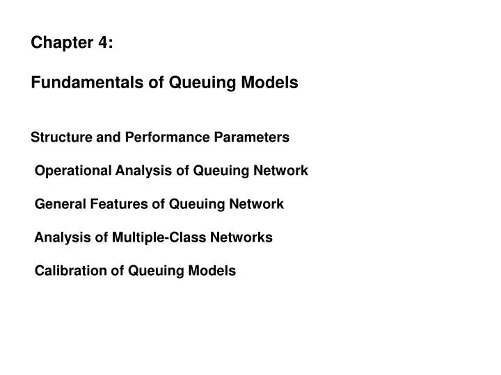
Chapter 4: Fundamentals of Queuing Models Structure and Performance Parameters Operational Analysis of Queuing Network General Features of Queuing Network Analysis of Multiple-Class Networks Calibration of Queuing Models.

E N D
Chapter 4: Fundamentals of Queuing Models Structure and Performance Parameters Operational Analysis of Queuing Network General Features of Queuing Network Analysis of Multiple-Class Networks Calibration of Queuing Models
4.1 Structure and Performance Parameters-A queuing network model (QNM) of a computer system is a collection of service stations connected via directed paths along which the customers of the system move.-The stations represent various system resources. And the customers represent jobs, processes, or other active entities. -The customers move from one station to another, queuing up at each for some service. The service requirement of a customer at a station is a random variable that is described by a probability distribution. -In general, a QNM may also have some special types of stations, such as those involved in resource allocation and deallocation ;
4.1 Structure and Performance Parameters-A queuing network model (QNM) of a computer system is a collection of service stations connected via directed paths along which the customers of the system move.-The stations represent various system resources. And the customers represent jobs, processes, or other active entities. -The customers move from one station to another, queuing up at each for some service. The service requirement of a customer at a station is a random variable that is described by a probability distribution. -In general, a QNM may also have some special types of stations, such as those involved in resource allocation and deallocation ;
4.1.1 Open and Closed Models -A QNM in which there is no restriction on the number of customers is called an open or infinite population model. -In such models, the customers initially arrive from an external source and eventually leave the system. -Fig. 4-1 shows an example of an open model. FIGURE 4-1 : An open model of a computer system.
-In models where the number of customers is fixed (i.e., no arrivals from, or departures to, the external world), the model is called a closed or limited population model with the number of circulating customers known as the population. -In a closed model, the arrival rate to any station must drop to zero if all circulating customers are already queued up at that station. -Fig. 4-2 shows an example of a closed model.
-We call a QNM well-formed if it is connected and has a well-defined long-term behavior. -We defer the details concerning this property to section 4.4.1 and only state the results for simple QNM's. -A closed QNM is well-formed if every station is reachable from all others with a nonzero probability. -The same definition applies to an open, connected QNM if we add a hypothetical station H that generates all external arrivals and absorbs all departing customers. -We shall henceforth assume that all QNM's that we consider are well-formed.
4.1.2 performance parameters -A simple QNM requires the following inputs: (a) number of stations, henceforth denoted as M, (b) service-time distribution and scheduling discipline at each station, (c) routing probabilities of customers among stations, and (d) population (for closed models) or interarrival-time distribution (for open models). -The output parameters of interest are the various performance measures at each station, such as response time, queue length, throughput, and utilization.
-In the following list, we define certain basic input and output parameters for the stations of a simple queuing network and establish notations for them. • Average service time Si : Average time spent in serving a customer at station i. We shall often speak of the (average) service rate, denoted µi This is defined as simply 1/si 2. External arrival rate Λi : Average rate at which customers arrive to station i, from the external world. This applies to open networks only. 3. Routing probability qij : Fraction of departures from station i headed to station j next.
4. Throughput λi or λi(N): Average number of service completions per unit time at station i. 5. Average response time Ri or Ri (N): Average time a customer spends at station i, either waiting to be served or receiving service. 6. Average waiting time Wi or Wi (N): Average time a customer spends at station i waiting to be served. 7. Average queue length Qi or Qi(N): Average number of customers at station i, including those being serviced. -8. Average waiting line length Li or Li(N): Average number of customers at station i, excluding those being serviced. -9. Utilization Ui or Ui(N): Fraction of time that station i is busy. (As such, this definition applies only when si is independent of n: a more general definition is introduced in Section 4.3.2).
10.Queu-length distribution pi(n) or pi(n|N) : Probability of finding n customers at station i.(Notice the | separating n and N.) 4.2 Operational Analysis of Queuing Models -In this section, we derive several relationships between various performance parameters. -We shall use the operational approach for deriving these, rather than the stochastic approach. -In the operational approach, we deal with behavior sequences and their properties, rather than with random processes. 4.2.1 Behavioral Properties -suppose that we observe a queuing system for a time period T and record all interesting events (arrivals and service completions at each station) during this period.
- There are three properties of particular interest concerning such a behavior sequence: -homogeneity, -flow balance, -and one-step behavior -The concept of homogeneity applies to arrivals, services, and routing. -Homogeneous arrivals means that the average arrival rate to a station is independent of the number of customers present there. -Similarly, homogeneous service means that the average service rate is independent of the number of customers at the station. -Note that the service rate must be zero when the station is empty,
-and in a closed network, the arrival rate must drop to zero when all N customers are present at the station. -The definition of homogeneity does permit this essential form of dependence. -Routing homogeneity means that the routing probabilities do not depend on the number of customers present at the source, destination, or any other station. -We shall implicitly assume routing homogeneity throughout this section. -Flow balance. refers to the property that the total number of arrivals to a station during the period T equals the total number of departures from the station.
Flow balance is an appropriate assumption in most situations, and is essential for studying the long –term behavior of the system. -One-step behavior means that - (a) arrivals do not coincide with departures, and • (b) at any instant, only one arrival or one departure can occur. -As an example, consider the behavior sequence shown in Fig. 4-3 for a station in a closed system with a population of three. FIGURE 4-3 : A sample behavior sequence.
-Here the upward transitions indicate arrivals, and the downward transitions indicate departures. -Thus, the vertical axis gives the number of customers present in the system. • The labels on the horizontal segments show the time units for which the system stays in the corresponding state. 4.2.2 Operational Definitions of Performance Measures -Suppose that the system of interest is station i belonging to a closed network with population N. -Let us define the following parameters over the observation period T:
-Ai (n) Number of arriving customers who find n customers at station i. -Di (n) Number of departing customers who leave behind n-1 customers at station i (i.e., the number of departures while the station is in state n). -Ti(n) Duration of time for which there are n customers at station i. -Note that Ai(N)=0 and Di(0)=0, but Ti(n) may be nonzero for all values of n € 0..N.Let Bi denote the total busy period. Obviously,
-Let Ai and Di denote, respectively, the total number of arrivals and departures during time T. Then n=0n=1 (2.2) -Let Xi(N) denote the overall arrival rate to station i. Then, Xi(N) = Ai|T (2.3) -Let Yi (n| N) denote the arrival rate to station i when n customers are present there. This is often known as restricted arrival rate and is given by (2.4)
-Note that Yi(N|N)=0. The departure rate or throughput of station i, denoted λi(N), is given by λi(N) = Di|T (2.5) The average service time of station i when n customers are present there, denoted si (n), is given by (2.6) -In analogy with Yi(n| N), we can think of the service rate µi(n) as the restricted departure rate. - If the services are homogeneous, we denote si(n) and µi(n) as simply si and µi respectively.
-If the arrivals are homogeneous, Yi(n|N) is independent of n for n<N, and denoted as Yi(N). -Flow balance means that Ai=Di, which implies that Xi(N) = λi(N). -In a queuing system, there are three interesting distributions of the number of customers present at a station: • Distribution seen by an arriving customer, denoted PAi(.|.). By definition, the probability that an arriver finds n customers in the system is given by PAi(n| N) = Ai(n) / Ai for 0≤ n<N(2.7) • Distribution seen by a departing customer, denoted PDi(.׀.).The probability that a departer
leaves behind n customers in the system is given by PDi(n| N) = Di(n+1) / Di for 0≤ n<N(2.8) Distribution seen by a random observer, denoted Pi(.|.). This is the fraction of time the system contains n customers, and is given by pi(n| N) = Ti(n) / T for 0≤ n≤N(2.9) - We shall see detailed relationships involving these distributions in sections 4.2.4 and 4.2.5. -As a simple example, the utilization Ui(N), as defined earlier, can be expressed as (2.10)
4.2.3 Forced Flows and Visit Ratios -This section concerns the analysis of queuing networks operating under flow balance. -This is the most frequently encountered situation in practice, and we shall show how the throughputs of all stations can be related in such a case. -These results hold in stochastic systems as well, if we examine their steady –state behavior The results follow from a simple conservation property, often known as the forced-flow law, which states that at any branch or join point in a network, there is no net accumulation or loss of customers. -Let λi denote the throughput of station i in a flow- balanced network with M stations
-Then for any station i, the total arrival rate should also be λi. -This arrival rate can be expressed in terms of the throughputs of other stations by accounting for all the flows into station i. -This gives (2.11) -where Λi is the external arrival rate to station i, and qji is the probability that a customer exiting station j goes to station i directly. -We can put these equations in the following matrix form A . λ = Λ (2.12) - where A is a M×M matrix of qij's, and λ and Λ are M×1 vectors of λi 's and Λi 's respectively.
-If the network is open, the system (2.12) is nonhomogeneous, and will have a unique solution so long as the network is well-formed. -Because throughput ratios can be determined easily in both open and closed networks, -it is convenient to introduce the notion of relative throughputs or visit ratios. -The reference station for computing these ratios can be chosen arbitrarily, -since the results will be independent of this choice. -We shall denote the visit ratio for station i as vi. -By definition, for any two stations i and j, vi / vj = λi / λj(2.13)
-If station k is chosen as the reference station, we can also interpret vi as the number of visits to station i for each visit to station k. -As we shall see in later chapters, visit ratios often provide adequate information to calibrate and solve a model, and the routing probabilities are not needed Example 4.1 Compute the relative throughputs for each station in figures 4-1 and 4-2 respectively. Solution Let Λ denote the external arrival rate, and λi the throughput of station i. -Then for Fig. 4-1, we can write the following equations λ1 = Λ + λ2 + λ3 λ2 = (1-p) λ1× q λ3 = (1-p) λ1× (1-q)
-Suppose that we define visit ratios relative to the external source, i.e., vi =λi /Λ. -Then the equations above yield the following solution: v1 = 1/p v2 = q(1-p)/p and v3 =(1-q)(1-p)/p -Note that here we can determine exact throughputs. -For example, if p=0.1, q=0.8, and Λ=10/sec, then λ1=100/sec, λ2=72/sec, and λ3= 18/sec. -For the model of Fig. 4-2, we have λ2 = λ1 + (1-p)( λ3 + λ4 ), λ3 = qλ2 , λ4 = (1-q) λ2 -It is easy to see that these equations are linearly independent, but we cannot write any more independent equations. -Thus, exact throughputs cannot be determined, but visit ratios can.
-For example, if we let v2=1, p= 0.2, and q=0.6, then v1= 0.2, v3= 0.6, and v4= 0.4. 4.2.4 Some Fundamental Results -In this section we prove three important operational relationships. • which hold under very general conditions. -We start with a simple property known as the throughput law. -By the definition of throughput, we have -Put in standard form, the throughput law then states (2.14)
-Note that (2.14) would hold for any behavior sequence since its derivation does not need any assumptions (homogeneity, one-step behavior or flow balance). -In particular, throughput law would continue to hold even in the context of stochastic analysis, where we are dealing with the statistical properties of the system,instead of the observable properties of finite behavior sequences. - If the services are homogeneous, i.e., µi(n)=µ i for all n>0, (2.14) reduces to λi (N) = µi [ 1- pi (0|N)](2.15) -Using equation (2.10), we get Ui (N) = λi (N) si(2.16)
-This simple property is known as the utilization law. -It also holds in the stochastic sense, provided that the service rate is independent of the "load" at station i. -A more direct way of obtaining the utilization law is as follows: Throughput and service rate describe the behavior of a station on its "output end". - Quite analogously, arrival rate and restricted arrival rates describe the behavior on the "input end" of the station.
Thus, like the throughput law, we have the following arrival law. (2.17) • The proof follows trivially from the definition (without any assumptions). - Under flow balance, the arrival rate is the same as throughput, which means that equations (2.14) and (2.17) give two ways of expressing the throughput.
If the arrivals are homogeneous, i.e.,Yi(n| N)=Yi(N) for all n<N, equation(2.17) yields the following simple relationship. X i (N)=Yi(N)(1-Pi (N|N))(2.18) • Notice the complementary nature of equations (2.15) and (2.18). • A simple way to remember them is to note that services cannot occur if the station is empty, and arrivals cannot occur if the station is full. Next we discuss Little's law, which relates average response time to the average queue length. • Consider a closed region Ω enclosing some portion of a queuing network. • Let λΏ be the output rate (or throughput) of this region, • QΏ the average number of customers in the region, and • RΏ the average time spent by a customer inside the region.
-Then Littl's law states that λΏ . RΏ = QΏ (2.19) - Since Little's law applies to any closed region, we can obtain a number of interesting results by choosing this region in special ways. • For example, there are three ways to apply Littl's law to a single station i : • To the entire station, which gives Qi = λi Ri FIGUR 4-4 : Arrival and departure functions.
2. To only the waiting line at the station, which gives Li = λiWi . 3. To only the "service box" of the station. This ismost useful if the services are homogeneous. - In this case, the average number of customers in the "service box" is same as the probability that the server is busy, which in turn is the utilization. • Thus, we get the utilization law Ui = λi si . • 4.2.5. Properties of Queue Length Distributions If the arrivals (departures) occur singly, then. In any system state n, at most one arrival (departure) can remain unmatched by a departure (arrival). - This happens because the system cannot return to state n unless an opposite event occurs. -
It follows that Vn | Ai(n) - Di(n+1)| ≤ 1(2.23) - Where Di(n+1) can exceed Ai(n) only if we start with a nonempty system. - Under flow balance, we cannot have an arriver who has not departed, or vice versa, and hence equation (2.23) reduces to Ai(n)= Di(n+1). - This also implies Ai= Di , as expected. Thus, we get the important result that under flow balance and one-step behavior, the arriver's distribution is the same as that of the departer's, i.e., PAi(n| N)= PDi(n| N)(2.24) • We can also get recursive equations for random observer's and arriver's distributions under these two assumptions. By definition, - Where we have used the identity Di(n)= Ai(n-1).
- Recognizing various terms. We get Pi(n| N)= si(n) Yi(n-1 |N) Pi(n-1|N)(2.25) • Similarly, for the arriver's distribution we get - Which yields PAi(n| N)= si(n) Yi(n| N) PAi(n-1|N)(2.26) - We can show another interesting result popularly known as the arrival theorem. - It states that PAi(n| N)= Pi(n|N-1)(2.27) - That is, under flow balance and one-step behavior, an arriving customer sees the random observer's distribution with itself removed from the network.
-For a station in an open network that exhibits flow balance and one-step behavior, we have PAi(n)= Pi(n)= PDi(n) for all n . • The departer's distribution can be related to the random observer's distribution (without any assumptions) as follows: (2.28) - Under flow balance and one-step behavior, using (2.24) we get PAi(n| N)= µi(n+1) Pi(n+1| N) λi(N)(2.29) - Furthermore, using the arrival theorem, we get the so called marginal local balance theorem, which can be restated as µi(n) Pi(n|N)= λi(N) Pi(n-1|N-1)(2.30) - We shall prove this equation using stochastic means in section 7.2. - In practice, the arrivals are often homogeneous, and we can show some interesting results under this assumption.
-By definition - Therefore, by equation (2.18) we get the following relationship (without assuming one-step behavior or flow balance) (2.31) - That is, in a closed network under homogeneous arrivals, the arriver's distribution is a simple renormalization of the random observer's distribution. • For an open network, this equation means that the arriver's and random observer's distributions are identical . • If the system shows one-step behavior and flow balance as well, we can use .(2.29) to get (2.32)
-This recurrence relation, along with the requirement that all probabilities sum to 1, gives us the following expression for Pi(n| N) (2.33) Finally, under homogeneous services, flow balance, and one-step behavior, (but arrivals not necessarily homogeneous ), equation (2.29) reduces to Pi(n| N)= Ui(N) PAi(n-1|N) , • which means that
which along with little's law gives the following interesting relationship Ri(N) = si(1+ QAi(N)) (2.34) • where QAi(N) is the average queue length seen by an arriving customer. • Note that by the arrival theorem,QAi(N)=Qi(N-1) • This substitution gives us the well-known mean value theorem, which we shall prove using stochastic means in section 7.2. Example 4.2 characterize the behavior sequence shown in fig 4-3 and compute the three distributions for it. Solution we already noted that this behavior sequence is one-step and flow balanced.
The performance parameters corresponding to Fig. 4-3 can be computed using the relationships given above and are shown in Table 4.1. • Note that Ai = Di = 7 as expected from the flow balance property, which also means that the arrival rate Xi (N) and throughput λi(N) should be the same (=7/15 k). • Both arrivals and services are homogeneous since Yi (n|N) and si (n) are independent of n . • Note that the utilization law applies because Ui=1- Pi(0) =7/15 andsiλi = k .7/(15k) = 7/15. • Also PAi(n) is simply a renormalization of Pi(n), and • PDi(n)= PAi(n) as expected.
Comparison of Operational and Stochastic Analysis • behavioral sequences rather than random processes • behavioral properties rather than statistical properties • finite and infinite behavior sequence • In spite of this difference, under comparable assumptions, many of the results obtained from the two approaches are identical.
comparable assumptions: One-step behavior Flow balance homogeneity An operational assumption is a concrete property of a given behavioral realization, whereas the corresponding stochastic assumption is a statistical statement about all possible behavior sequences. Equating the two properties naively will often lead to incorrect conclusions. although operational analysis is useful in explaining stochastic results under exponential distributions.
In this section we briefly consider some extensions to simple QNM’s that are useful in modeling complex characteristics of real systems. We shall also indicate the level of difficulty in solving models containing these features. General Features of Queuing Network
A real computer system may serve many categories of jobs such that the level of service provided and/or routing depend on the category. Chain: permanent categorization of jobs; a job belonging to one chain cannot switch to another chain. Class: different phases in each chain Classes and Chains
There are many practical situations where the average service rate of a station depends on its loading level. suppose that station i contains k identical servers, each capable of serving at the average rate of µi0: µi(1) : basic service rate µi0. Ci(n) : Capacity Function and Ci(1)=1. Load-Dependent Stations
By the throughput law, we have: Now we define the utilization of station i as: Note: Ui(N) can be grater than 1. Load-Dependent Stations:Utilization
Let station i be either load-independent or a multiserver. In both cases, each customer requires the same amount of service time, independent of the load: Multiplying both sides by i and then applying Little’s Law: . Load-Dependent Stations:Utilization (Cont.)
Load-Dependent Stations:system response time as a function of number of terminals System Response Time Nvbsb- Saturation asymptote Horizontal asymptote (Minimum value of R) R(1) Number of Terminals N*
This curve has two asymptotes: When N=1: When N is sufficiently large, Let N* denote the abscissa of the intersection between the two asymptotes: Load-Dependent Stations:About former Fig.