Download
1 / 44
440 likes | 582 Views
Local & Adversarial Search. CSD 15-780: Graduate Artificial Intelligence Instructors: Zico Kolter and Zack Rubinstein TA: Vittorio Perera. Local search algorithms. Sometimes the path to the goal is irrelevant: 8-queens problem, job-shop scheduling circuit design, computer configuration

E N D
Local & Adversarial Search CSD 15-780: Graduate Artificial Intelligence Instructors: ZicoKolter and Zack Rubinstein TA: Vittorio Perera
Local search algorithms • Sometimes the path to the goal is irrelevant: • 8-queens problem, job-shop scheduling • circuit design, computer configuration • automatic programming, automatic graph drawing • Optimization problems may have no obvious “goal test” or “path cost”. • Local search algorithms can solve such problems by keeping in memory just one current state (or perhaps a few).
Advantages of local search • Very simple to implement. • Very little memory is needed. • Can often find reasonable solutions in very large state spaces for which systematic algorithms are not suitable.
Problems with hill-climbing • Can get stuck at a local maximum. • Cannot climb along a narrow ridge when each possible step goes down. • Unable to find its way off a plateau. Solutions: • Stochastic hill-climbing – select using weighted random choice • First-Choice hill-climbing – randomly generate neighbors until one better • Random restarts – run multiple HC searches with different initial states.
Simulated Annealing Search • Based on annealing in metallurgy where metal is hardened by heating to high state and cool gradually. • The main idea is to avoid local maxima (or minima) by having a controlled randomness in the search that gradually decreases.
Beam Search • Like hill-climbing but instead of tracking just one best state, it tracks k best states. • Start with k states and generate successors • If solution in successors, return it. • Otherwise, select k best states selected from all successors. • Like hill-climbing, there are stochastic forms of beam search.
Genetic Algorithms • Similar to stochastic beam search, except that successors are drawn from two parents instead of one. • General idea is to find a solution by iteratively selecting fittest individuals from a population and breeding them until either a threshold on iterations or fitness is hit.
Genetic algorithms cont. • An individual state is represented by a sequence of “genes”. • The selection strategy is randomized with probability of selection proportional to “fitness”. • Individuals selected for reproduction are randomly paired, certain genes are crossed-over, and some are mutated.
Genetic algorithms cont. • Genetic algorithms have been applied to a wide range of problems. • Results are sometimes very good and sometimes very poor. • The technique is relatively easy to apply and in many cases it is beneficial to see if it works before thinking about another approach.
Adversarial Search • The minimax algorithm • Alpha-Beta pruning • Games with chance nodes • Games versus real-world competitive situations
Adversarial Search • An AI favorite • Competitive multi-agent environments modeled as games
From single-agent to two-players • Actions no longer have predictable outcomes • Uncertainty regarding opponent and/or outcome of actions • Competitive situation • Much larger state-space • Time limits • Still assume perfect information
Formalizing the search problem • Initial state = initial game/board position and player • Successors = operators = all legal moves • Terminal state test (not “goal”-test) = a state in which the game ends • Utility function = payoff function = reward • Game tree = a graph representing all the possible game scenarios
What are we searching for? • Construct a “strategy” or “contingent plan” rather than a “path” • Must take into account all possible moves by the opponent • Representation of a strategy • Optimal strategy = leads to the highest possible guaranteed payoff
The minimax algorithm • Generate the whole tree • Label the terminal states with the payoff function • Work backwards from the leaves, labeling each state with the best outcome possible for that player • Construct a strategy by selecting the the best moves for “Max”
Minimax algorithm cont. • Labeling process leads to the “minimax decision” that guarantees maximum payoff, assuming that the opponent is rational • Labeling can be implemented using depth-first search using linear space
Illustration of minimax MAX MIN 3 3 2 2 3 12 8 2 4 6 14 5 2
But seriously... • Can’t search all the way to leaves • Use Cutoff-Test function; generate a partial tree whose leaves meet the cutoff-test • Apply heuristic to each leaf • Assume that the heuristic represents payoffs, and back up using minimax
What’s in an evaluation function? • Evaluation function assigns each state to a category, and imposes an ordering on the categories • Some claim that the evaluation function should measure P(winning)...
Evaluating states inchess • “material” evaluation • Count the pieces for each side, giving each a weight (queen=9, rook=5, knight/bishop=3, pawn=1) • What properties do we care about in the evaluation function? • Only the ordering matters
Evaluating states inbackgammon Possible goals (features): • Hit your opponent's blots • Reduce the number of blots that are in danger • Build points to block your opponent • Remove men from board • Get out of opponent's home • Don't build high points • Spread the men at home positions
Learning evaluation functions • Learning the weights of chess pieces... can use anything from linear regression to hill-climbing. • The harder question is picking the primitive features to use.
Problems with minimax • Uniform depth limit • Horizon problem: over-rates sequences of moves that “stall” some bad outcome • Does not take into account possible “deviations” from guaranteed value • Does not factor search cost into the process
Minimax may be inappropriate… MAX MIN 99 100 99 1000 1000 1000 100 101 102 100
Reducing search cost • In chess, can only search full-width tree to about 4 levels • The trick is to “prune” certain subtrees • Fortunately, best move is provably insensitive to certain subtrees
Alpha-Beta pruning • Goal: compute the minimax value of a game tree with minimal exploration. • Along current search path, record best choice for Max (alpha), and best choice for Min (beta). • If any new state is known to be worse than alpha or beta, it can be pruned. • Simple example of “meta-reasoning”
Illustration of Alpha-Beta 11 10 11 48 10 11 10 11 9 10 48
Implementation of Alpha-Beta function Alpha (state, , ) if Cutoff (state) then return Value(state) for each s in Successors(state) do Max(, Beta (s, , )) if then return end return
Implementation cont. function Beta (state, , ) if Cutoff (state) then return Value(state) for each s in Successors(state) do Min(, Alpha (s, , )) if then return end return
Effectiveness of Alpha-Beta • Depends on ordering of successors. • With perfect ordering, can search twice as deep in a given amount of time (i.e., effective branching factor is SQRT(b)). • While perfect ordering cannot be achieved, simple heuristics are very effective.
What about time limits? • Iterative deepening (minimax to depths 1, 2, 3, ...) • Can even use iterative deepening results to improve top-level ordering
Games with an element of chance • Add chance nodes to the game tree • Use the expecti-max or expecti-minimax algorithm • One problem: evaluation function is now scale dependent (not just ordering!) • There is even an alpha-beta trick for this case
State-of-the-art programs Chess:Deep Blue [Campbell, Hsu, and Tan; 1997] • Defeated Gary Kasparov in a 6-game match. • Used parallel computer with 32 PowerPCs and 512 custom VLSI chess processors. • Could search 100 bilion positions per move, reaching depth 14. • Used alpha-beta with improvements, following “interesting” lines more deeply. • Extensive use of libraries of openings and endgames.
State-of-the-art programs • Checkers: [Samuel, 1952] • Expert-level performance using a 1KHz CPU with 10,000 words of memory. • One of the early example of machine learning. • Checkers:Chinook [Schaeffer, 1992] • Won the 1992 U.S. Open and first to challenge for a world championship. • Lost in match against Tinsley (World champion for over 40 years who had lost only in 3 games before match). • Became world champion in 1994. • Used alpha-beta search combined with a database of all 444 bilion positions with 8 pieces or less on board.
State-of-the-art programs Backgammon:TD-Gammon [Tesauro, 1992] • Ranked among the top three players in the world. • Combined Samuel’s RL method with neural network techniques to develop a remarkably good heuristic evaluator. • Used expecti-minimax search to depth 2 or 3.
State-of-the-art programs Bridge:GIB [Ginsburg, 1999] • Won computer bridge championship; finished 12th in a field of 35 at the 1998 world championship. • Examine how each choice works for a random sample of the up to 10 million possible arrangements of the hidden cards. • Used explanation-based generalization to compute and cache general rules for optimal play in various classes of situations.
Lots of theoretical problems... • Minimax only valid on whole tree • P(win) is not well defined • Correlated errors • Perfect play assumption • No planning