Download

1 / 13
130 likes | 137 Views
An evolutionary computing approach to minimize dynamic hedging error. Saeid Nahavandi School of Eng and Information Technology Deakin University, Australia. Mohammad Khoshnevisan School of Accounting & Finance Griffith University, Australia.

E N D
An evolutionary computing approach to minimize dynamic hedging error Saeid Nahavandi School of Eng and Information Technology Deakin University, Australia Mohammad Khoshnevisan School of Accounting & Finance Griffith University, Australia
Problem of endogenous capital guarantee • Let a structured financial product be made up of an envelope of J different assets such that the investor has the right to claim the return on the best-performing asset out of that envelope after a stipulated lock-in period • Then, if one of the J assets in the envelope is the risk-free asset then the investor gets assured of a minimum return equal to the risk-free rate i on his invested capital at the termination of the stipulated lock-in period • This effectively means that his or her investment becomes endogenously capital-guaranteed as the terminal wealth, even at its worst, cannot be lower in value to the initial wealth plus the return earned on the risk-free asset minus a finite cost of portfolio insurance, which is paid as the premium to the option writer
Expected payoff from a multi-asset capital guaranteed structured financial product • The expected present value of terminal option payoff is obtained as follows: Ê (r) t=T = Max [w, Max j {e-it E (rj) t=T}], j = 1, 2 … J – 1 In the above equation, i is the rate of return on the risk-free asset and T is the length of the investment horizon in continuous time and w is the initial wealth invested i.e. ignoring insurance cost, if the risk-free asset outperforms all other assets then we get: Ê (r) t=T = weiT/eiT = w • Now what is the probability of each of the (J – 1) risky assets performing worse than the risk-free asset? Even if we assume that there are some cross-correlations present among the (J – 1) risky assets, given the statistical nature of the risk-return trade-off, the joint probability of all these assets performing worse than the risk-free asset will be very low over even moderately long investment horizons. And this probability will keep going down with every additional risky asset added to the envelope. Thus this probability can become quite negligible if we consider sufficiently large values of n
Formulation as a generalized stochastic optimization model • For an option writer who is looking to hedge his or her position, the expected utility maximization criterion will require the tracking error to be at a minimum at each point of rebalancing, where the tracking error is the difference between the expected payoff on the best-of option and the replicating portfolio value at that point • At each point of re-balancing, the tracking error has to be minimized if the difference between the expected option payoff and the replicating portfolio value is to be minimized. The more significant this difference, the more will be the cost of re-balancing associated with correcting the tracking error; and as these costs cumulate; the less will be the ultimate utility of the hedge to the option writer at the end of the lock-in period. Then the cumulative tracking error over the lock-in period is given as: = t |E (rt) – vt| • Here E (r) t is the expected best-of option payoff at time-point t and vt is the replicating portfolio value at that point of time. Then the replicating portfolio value at time t is obtained as the following linear form: vt = (p0) t eit + j {(pj) t (Xj) t}, j = 1, 2 … J – 1 • Here (Xj) t is the realized return on asset j at time-point t and p1, p2 … pJ-1 are the respective allocation proportions of investment funds among the J – 1 risky assets at time-point t and (p0) t is the allocation for the risk-free asset at time-point t. Of course: (p0) t = 1 – j (pj) t • It is the portfolio weights i.e. the p0 and pj values that are of critical importance in determining the size of the tracking error. The correct selection of these portfolio weights will ensure that the replicating portfolio accurately tracks the option
Casting the objective function as the total cost of tracking error • The problem of minimizing the randomness associated with the tracking error can be mathematically cast as a sequential, stochastic optimization problem with respect to the portfolio weight vector pt-1T corresponding to the last rebalancing time point. The latter rebalancing decisions are affected by the earlier decisions and also by the randomness or white noise component in the market information. The squared cost of tracking error for the tth rebalancing is obtainable as follows: [C (t)] 2 = [htδt + Maxj E (rj) t – pt-1TRt] 2 • Here ht is a fixed rebalancing cost and δt is a binary variable such that δt = 1 when [Maxj E (rj) t – ptTRt] > ht and δt = 0 otherwise. That is, it will be feasible to rebalance at time point t only if the rebalancing cost at time point t is less than the cost of keeping the same portfolio weights as at time point t–1. Rt is the vector of expected returns on the J assets constituting the portfolio
Mathematical formulation of the generalized optimization model • Let the probability density function for getting a specific vector p tT be given by t. Then over a period of t = 1, 2 ... T time points, this is obtainable as the joint conditional likelihood function obtainable as follows: t [ (ptT | pt-1T)] = (pTT | pT-1T) (pT-1T| pT-2T) ... (p2T | p1T) (p1T) Therefore the expected squared cost of tracking error is obtainable as follows: E [C (t)] 2 = ∫ ... ∫ [t { (ptT | pt-1T)}] [htδt + {Maxj E (rj) t – pt-1TRt} 2] dp1T... dpTT • The target is to minimize this expected squared cost of tracking error over the entire investment horizon i.e. for all t = 1, 2 ... T. To allow the replicating portfolio to be self-financing, the elements of ptT must be unrestricted in sign • The fundamental stochastic recurrence relations to be computed in the minimization procedure are obtainable using the standard derivation as follows: Ft* (st+1) = Mint Σ t Qt {st, ptT, E [C (t)] 2}, 1 ≤ t ≤ T, where Qt {st+1, ptT, E [C (t)] 2} = Rect {st+1, ptT, E [C (t)] 2} + F*t-1, 2 ≤ t ≤ T and Q1 {s2, p1T, E [C (1)] 2} = Rec1 {s2, p1T, E [C (1)] 2} In the above minimization procedure introduction of random variables causes no increase in the number of state variables. Since Qt is a function of only one random variable E [C (t)] 2, only one parameter at a time is introduced into the minimization procedure. This helps to reduce the considerable difficulties associated with multi-variate sequential optimization
Developing a Genetic Algorithm model as a computational alternative • Given a necessarily biological basis of the evolution of utility forms (Robson, 1968; Becker, 1976), a haploid genetic algorithm model, which, as a matter of fact, can be shown to be statistically equivalent to multiple multi-armed bandit processes (Berry and Fristedt, 1985), should show satisfactory convergence with the Black-Scholes type expected utility solution to the problem of minimizing the target cost function. This would allow for estimation of the optimal weight vector ptT without explicitly solving the stochastic optimization problem outlined above • A computational haploid genetic algorithm model has been programmed for this purpose in Borland C; Release 5.02 and performs the three basic genetic functions of reproduction, crossover and mutation with the premise that in each subsequent generation x number of chromosomes from the previous generation will be reproduced based on the principal of natural selection (De Jong, 1976). The model is presently restricted to n = 3 underlying assets within the structured financial product • Following the reproduction function, 2(x – 1) number of additional chromosomes will be produced through the crossover function, whereby every g th chromosome included in the mating pool will be crossed with the (g + 1) th chromosome at a pre-assigned crossover locus. There is also a provision in the computer program to introduce a maximum number of mutations in each current chromosome population in order to enable rapid adaptation
A proposed haploid Genetic Algorithm model • According to our proposed haploid genetic algorithm reproduction and crossover functions, the size of the nth generation i.e. the number of chromosomes in the population at the end of the nth generation is given by the following first-order, linear difference equation: Gn = Gn – 1 + 2 (Gn – 1 – 1) = 3 Gn – 1 – 2 • If x initial number of chromosomes are introduced at n = 0, we have G0 = x. Then, obviously, G1 = x + 2(x – 1) = 3x – 2 = 31 (x – 1) + 1. Extending the recursive logic to G2 and G3 we therefore get G2 = 9x – 8 = 32 (x – 1) + 1 and G3 = 27x – 26 = 33 (x – 1) + 1. Thus, extending to Gt we can write the following relation: Gt = 3t (x – 1) + 1 • Therefore, Gt+1 = 3t+1 (x – 1) + 1. But Gt+1 = 3Gt – 2. Substituting for Gt we thereby get, Gt+1 = 3{3t (x – 1) + 1} – 2 = 3t+1 (x – 1) + 3 – 2 = 3t+1 (x – 1) + 1. Therefore the case is proved for Gt+1. But we have already proved it for G1, G2 and G3. Therefore, by the principle of mathematical induction, the general formula is derived as follows: Gn = 3n (x – 1) + 1 • This simple genetic algorithm performs satisfactorily in terms of computational efficiency as well as the target minimization objective for n = 3. However, to reduce computational complications at the onset we have ignored a part of the objective function i.e. htδt. However our proposed computational genetic algorithm model may be appropriately extended to cover the complete version of the stochastic optimization problem with the minimization of the expected squared cost of tracking error as the target
A 2-asset numerical illustration • The following table shows the hypothesized figures relating to the two correlated risky assets and the risk-free asset underlying the best-of option as have been used in computing the expected option pay-offs. These figures have been chosen so as to maximize the chances for a pay-off pattern whereby each of the risky assets may be seen to outperform the other for some length of time within the 12-month lock-in period • A Monte Carlo simulation algorithm was used to generate the potential payoffs for the option on best of three assets at the end of each month for t = 0, 2 … 11. The word potential is crucial in the sense that our option is essentially European and path-independent i.e. basically to say only the terminal payoff counts. However the replicating portfolio has to track the option all through its life in order to ensure an optimal hedge and therefore we have evaluated potential payoffs at each t • The potential payoffs from the option were computed as Max [(S1) t – (S0) t, (S2) t – (S0) t, 0]. The risky returns S1 and S2 were assumed to evolve over time following the stochastic diffusion process of a geometric Brownian motion (Stultz, 1982). The risk-free return S0 was continuously compounded approximately at a rate of 0.41% per month giving a 5% annual yield. We ran our Monte Carlo simulation model with the hypothetical data in Table 1 over a one-year lock-in period and calculated the potential option payoffs
Numerical results • For an initial input of $1, apportioned at t = 0 as 45% between S1 and S2 and 10% for S0, we have constructed five replicating portfolios according to a simple rule-based logic: k% of funds are allocated to the observed best performing risky asset and the balance (90 – k) % to the other risky asset (keeping the portfolio self-financing after the initial investment) at every monthly re-balancing point. We have reduced k by 10% for each portfolio starting from 90% and going down to 50%. This simple hedging scheme performed quite well over the lock-in period when k = 90% but the performance falls away steadily as k is reduced every time. The cumulative tracking errors corresponding to choices of k are given in the following table:
Numerical results … continued What we have done next is to introduce the above choices of k into our haploid genetic algorithm model encoded in the form of bit strings as the initial chromosomes. Subsequently we have noted the dominance of chromosomes in the range 80 < k* 90 after three generations. The output of our genetic algorithm model is graphically depicted below:
Adaptation of Evolutionary Optimization Parameters Based on a Fuzzy Logic Controller • Our computational result as obtained above does provide some experimental support to the premise that embedding a Black Scholes type of expected payoff (utility) maximization function indeed results in evolutionary optimality (Robson, 2001) • Evolutionary optimization algorithms like a genetic algorithm principally work by trying to optimally prioritize between exploitation (existing knowledge) and exploration (new knowledge). One of the primary goals in an evolutionary optimization set-up is to avoid getting stuck in local optima (premature convergence) in the effort to optimally prioritize between exploitation and exploration. As the knowledge base (existing as well as new) often consists of vague and imprecise information, the genetic algorithm performance can be better controlled using fuzzy logic controllers (FLCs). The FLC control process allows for an ideal man-machine interface for the optimal prioritization between exploitation and exploration • The principal goal is to use an FLC with an input that is any combination of the genetic algorithm performance measures e.g. in our 3-asset dynamic hedging problem, it could very well be the mean square tracking error of the replicating portfolio. In a feedback control mechanism, the current performance measure of the genetic algorithm are routed through the FLC which computes new control parameter values that will be subsequently fed into the genetic algorithm. Standard genotype diversity measures like Hamming Distance, Euclidian Distance and entropy measures are also possible input candidates for the FLC along with common phenotype diversity measures like the span measure; span = [1/(N-1)Σ (fi – f*)2]½ [1/nΣfi]-1 for any pre-defined fitness criteria fi and the average fitness criterion f*
Extension of the proposed evolutionary optimization scheme for the 3-asset dynamic hedging problem using a simple FLC The genetic algorithm we have used here to solve the stochastic optimization problem of minimizing the option tracking error becomes particularly susceptible to getting stuck in local optima especially when the return on the risky assets underlying the best-of option have temporally unstable correlation and volatility. Especially for many of the longer term options; implied volatility measures are often based on subjective and imprecise probability assessments which can significantly slow down the search speed (Xu and Vukovich, 1993). Genetic algorithms controlled by FLCs can resolve the imprecise information dynamically during run-time thereby allowing faster adaptation (Herrera et. al., 1994). In the context of our 3-asset dynamic hedging problem, a fuzzy rule pseudocode could be implemented as follows: IF [r1 – MAX (r0, r1, r2)] 2 is <small> THEN raise k <slightly> ELSE lower k <slightly> The actual computational implementation of a FLC based genetic algorithm then becomes the immediate step to advance in the direction we have shown