Download
1 / 34
340 likes | 434 Views
D 1 -D 2 lifetime difference using D 0 K K , D 0 and D 0 K . W. Lockman, C. Chavez, J. Coleman, R. Cowan, K. Flood, B. Petersen BaBar Physics Workshop June 30 - July 2, 2008. Introduction Analysis Fit results Cross checks and validations Systematics.

E N D
D1-D2 lifetime difference usingD0KK, D0and D0K W. Lockman, C. Chavez, J. Coleman, R. Cowan, K. Flood, B. Petersen BaBar Physics Workshop June 30 - July 2, 2008 Introduction Analysis Fit results Cross checks and validations Systematics
A. Petrov, HEP-PH/0611361 Introduction • Mixing among the lightest neutral meson flavor eigenstates provides important information about • electroweak interactions, including CP violation • the CKM matrix • mixing loop virtual constituents • D0 system exhibits the smallest mixing • Short distance Standard Model (SM) suppression: • D mixing loop involves down-type quarks • b quark loop suppressed: • s and d quark loops GIM suppressed • mass difference amplitude O(10-5) or less • long distance mixing amplitudes predominant but hard to quantify W. Lockman
Mixing between Flavor States Schroedinger eqn governs time evolution (off diagonal M and elements determine mixing) • Flavor eigenstates can mix through weak interaction: • Mass eigenstates D1 and D2 ≠ flavor eigenstates • If weak interaction splits the masses or widths of mass eigenstates, flavor state mixing will occur,as seen from the time evolution: • mixing parameters: D1 = CP D2 = CP In the limit of CP conservation: W. Lockman
Mixing Observable • This analysis measures the lifetimes of • Cabibbo favoredD0K(CF) and • singly Cabibbo suppressedD0KKSCSdecays • This allows a determination of by measuring • In the limit of CP conservation, • No D* flavor tag used: • Higher background to signal than in the tagged analysis, but 4x the statistics • compared to tagged analysis, expect smaller statistical, larger systematic errors • No measurement of CP violating quantity, Y • Construct the untagged sample to be disjoint from the tagged sample • allows tagged and untagged results to be “trivially” combined W. Lockman
Previous yCP Measurements • yCP world average from HFAG A. Schwartz, arXiv:0803.0082 540 /fb tagged (BELLE) 384 /fb tagged and 91 /fb untagged (BaBar) (1.132 0.266)% W. Lockman
Previous Mixing Measurements • Best evidence for D0-D0 mixing to date (mainly BaBar, BELLE and CDF): yCP= (1.132 0.266)% consistent? (y includes yCP) W. Lockman
Untagged Analysis Strategy • Samples: • Untagged D0K • Untagged D0KK • Systematics considerations: • signal systematics correlated and mostly cancel in yCP • background composition different between samples • background systematics do not cancel in yCP • restrict sample to narrow D0 mass region symmetric about D0 peak: • 1.8495 < D0 < 1.8795 GeV/c2 • estimate background from sideband regions: • 1.81 < D0 < 1.83 GeV/c2 and 1.90 < D0 < 1.92 GeV/c2 • Background composition: • mainly combinatoric, small admixture of broken charm decays removed events containing a D* tagged decay W. Lockman
Untagged Selection • Selection requirements • tracks from a common point • KLHTight, piLHTight PID selectors • D0 invariant mass m, reconstructed decay time t and its error tfrom beam constrained TreeFitter vertex fit • P(2) > 0.1% • 1.80 < m < 1.93 GeV/c2 • -25 < t < 25 psec • t < 0.5 psec • Remove B decays using D0 center of mass momentum cut • P* >2.5 GeV/c • D0 daughter track number of DCH hits • NDCH ≧ 12 • Reduce uds backgrounds using helicity angle (angle between track in D0 rest frame and D0 boost direction) cut: • |cosh| < 0.7 • Remove events containing a selected D* tagged D0, K∓, KKdecay • For multiple D0 candidates sharing tracks, keep the one with highest P(2) W. Lockman
signalband sideband sideband sideband signalband sideband 2008 untagged analysis Data yields and purity in 1.8495 < m < 1.8795 GeV/c2 K KK W. Lockman
Untagged Analysis Fit Strategy Perform fit in stages to determine lifetimes of D0Kand D0KK decays • Fit D0 invariant mass distribution to determine signal yields in signal band • Background decay time fit: • D0 sidebands fit to determine dominant combinatorial background • use MC to determine signal and charm decay time distributions in sidebands • signal region backgrounds: • charm component from MC • combinatorial shape and yield parameters: weighted average from sidebands • Signal decay time fit: • Signal decay time PDF: • Exponential convolved with triple Gaussian with common offset t0 and scaled event-by-event errors • Two different signal fits: • baseline combined fit to K and KK samples with shared resolution function parameters • scale KK width relative to K • independent fits to K and KK samples with independent resolution parameters • signal region decay time error histogram PDFs: • combinatorial decay time error: summed distribution from sidebands • Combinatorial total decay time error = signal decay time error distribution W. Lockman
D0 Mass Data : MC Comparison • KK fit: • 2 Gaussians signal PDF • 2nd order polynomial background PDF • K fit: • 2 Gaussians+Bifurcated Gaussian signal PDF • 2nd order polynomial background PDF • Data-MC fit comparison: • disagreement between data and MC in sideband background yields • good agreement between data and MC in signal region background yields (next) K MC KK MC K data KK data W. Lockman
Data : MC Mass Fit yields K MCTruth K yields agree to within 5% in the signal box MC fit Data fit KK MCTruth KK yields agree to within 2% in the signal box MC fit Data fit W. Lockman
KK MC combinatorial fits lower sideband upper sideband signal region double Gaussianwith common mean and CB function W. Lockman
K combinatorial fits lower sideband upper sideband signal region double Gaussianwith common mean and CB function W. Lockman
Comb. Fit Validation in Signal Region KK MC K MC • Signal region PDF parameters: weighted average of parameters from sidebands • Yields scaled to signal region yields • Weighted averaging of parameters gives a PDF which matches truth matched combinatorial distribution W. Lockman
KK MC Sideband Decay time fit lower Upper • Lower and upper sideband KK MC PDFs overlaid on Decay time distributions W. Lockman
K MC Sideband Decay time fit lower Upper • Lower and upper sideband K MC PDFs overlaid on Decay time distributions W. Lockman
MC Signal Region fits KK K • KK and K MC PDFs overlaid on Decay time distributions W. Lockman
Data Signal Region Fit KK K combined Independent fit results: Combined fit results: W. Lockman
Validation and Cross Checks • Perform unblinded fit to determine K lifetime • results are close to world average • Fit truth decay time Monte Carlo samples • no deviation seen from exponential • Compare resolutions between K and KK • (t-ttrue)/(SKK*t) distributions are universal with SK=1, SKK=1.018 • Compare fit to truth matched combinatorial distribution in signal region with PDF determined from weighted average of sideband fits • results are nearly identical • Compare combinatorial decay time error distributions from truth matched MC to distributions obtained from sidebands • results are nearly identical W. Lockman
Validations and Cross Checks • Fit reconstructed Monte Carlo samples • compare with lifetime from fitting MC truth lifetime • Problem: fit to KK to generic Monte Carlo sample indicates a possible bias or a cruel statistical fluctuation • both fitted and truth lifetimes are low, ~(409.6+0.6) fsec, dialed 411.6 fsec • Construct an independent sample using KK signal and generic MC for background • fitted and truth lifetime analysis still under investigation, but preliminary results indicate lifetimes are coming out a bit higher than dialed, ~412 fsec • Kp fitted and dialed lifetimes are consistent with each other W. Lockman
Fit procedure: Difference between combined and independent fits Difference between combined fits with and without mass dependence Signal systematics: Offset in combined signal fit Signal yield from mass fit Signal box position Signal box size Detector: SVT misalignment Beam spot Magnetic field uncertainties Background systematics: Combinatorial yield Sideband positions Sideband widths Charm yields in signal, sidebands Charm lifetime Selection: Decay time error selection Decay time selection Multiple overlapping candidates Systematic Sources Under Investigation • My Guess: • largest systematics in red • total systematic error: 1 to 2 fsec W. Lockman
Status of Untagged Analysis • Decay time fits have been validated on luminosity weighted cocktail MC • can reproduce the true lifetime to within 0.2-0.3 fs • Blind decay time fits to data are completed • statistical errors appear to be sensible • Systematic and cross check studies are underway • BAD 1876 is completed up to systematics • Still striving to have a preliminary result for ICHEP W. Lockman
Extra material W. Lockman
True decay time distributions MC Truth decay time distributions KK standard generic KK embedded generic • Dialed and post selection MCtruth lifetime comparisons: • Kgeneric • KK embedded • KK signal • KK generic KK signal sample K standard generic W. Lockman
Decay time pulls vs true lifetime Decay time pull (t-ttrue)/t of signal events in 1.80 < m < 1.93 GeV/c2 mass region KK K Decay time pulls consistent with no true decay time dependence W. Lockman
Scaled Pull Comparisons Kolmogorov comparisons of scaled pull = (t-ttrue)/(St) distributions Compare truth matched signal scaled pull distributions: • K from generic sample, SK = 1 • KK from signal Monte Carlo sample, SKK = 1.018 Scaled pull distributions statistically consistent with each other • KS probabilities are 25-45% • Motivates combined fit anzatz W. Lockman
Mass-lifetime correlation: Vertexing bias t-ttrue vs reconstructed D0 mass Cross over point: • (m, t-ttrue) = (mD0, 0) • same in all distributions Steeper dependence in KK than in K Tagged K Untagged generic K Untagged generic KK Untagged signal KK W. Lockman
Combinatorial Background Error distrib. W. Lockman
Signal Error Distribution W. Lockman
KK MC signal region decay time fit Combinatorialbackground Shape is taken from Weighted average of lower and Upper sidebands Charmbackground Shape and yields taken from MC Charm fit in Signal Region |truefitted| = 0.3 fs W. Lockman
K MC signal region decay time fit Combinatorialbackground Shape is taken from Weighted average of lower and Upper sidebands Charm background Shape and yields taken from MC Charm fit in Signal Region |truefitted| ≈ 0.2 fs W. Lockman
KK data signal region decay time fit Combinatorialbackground Shape is taken from Weighted average of lower and Upper sidebands Charm background Shape and yields taken from MC Charm fit in Signal Region Lifetime: xxx.xxx 1.26 fs KKtagged sample error: 1.8 fs untagged sample offset: -7.4 1.2 fs tagged sample offset: -4.8 fs W. Lockman
K data signal region decay time fit Combinatorialbackground Shape is taken from Weighted average of lower and Upper sidebands Charm background Shape and yields taken from MC Charm fit in Signal Region Lifetime: 409.88 0.36 fs Ktagged sample error: 0.7 fs untagged sample offset: -4.64 0.28 fs tagged sample offset: -4.8 fs W. Lockman