Download
1 / 31
310 likes | 390 Views
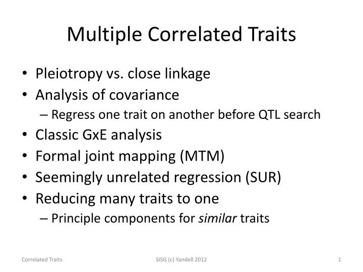
Multiple Correlated Traits. Pleiotropy vs. close linkage Analysis of covariance Regress one trait on another before QTL search Classic GxE analysis Formal joint mapping (MTM) Seemingly unrelated regression (SUR) Reducing many traits to one Principle components for similar traits.

E N D
Multiple Correlated Traits • Pleiotropy vs. close linkage • Analysis of covariance • Regress one trait on another before QTL search • Classic GxE analysis • Formal joint mapping (MTM) • Seemingly unrelated regression (SUR) • Reducing many traits to one • Principle components for similar traits SISG (c) Yandell 2012
co-mapping multiple traits • avoid reductionist approach to biology • address physiological/biochemical mechanisms • Schmalhausen (1942); Falconer (1952) • separate close linkage from pleiotropy • 1 locus or 2 linked loci? • identify epistatic interaction or canalization • influence of genetic background • establish QTL x environment interactions • decompose genetic correlation among traits • increase power to detect QTL SISG (c) Yandell 2012
Two types of data • Design I: multiple traits on same individual • Related measurements, say of shape or size • Same measurement taken over time • Correlation within an individual • Design II: multiple traits on different individuals • Same measurement in two crosses • Male vs. female differences • Different individuals in different locations • No correlation between individuals SISG (c) Yandell 2012
interplay of pleiotropy & correlation both pleiotropy only correlation only Korol et al. (2001) SISG (c) Yandell 2012
Brassica napus: 2 correlated traits • 4-week & 8-week vernalization effect • log(days to flower) • genetic cross of • Stellar (annual canola) • Major (biennial rapeseed) • 105 F1-derived double haploid (DH) lines • homozygous at every locus (QQ or qq) • 10 molecular markers (RFLPs) on LG9 • two QTLs inferred on LG9 (now chromosome N2) • corroborated by Butruille (1998) • exploiting synteny with Arabidopsis thaliana SISG (c) Yandell 2012
QTL with GxE or Covariates • adjust phenotype by covariate • covariate(s) = environment(s) or other trait(s) • additive covariate • covariate adjustment same across genotypes • “usual” analysis of covariance (ANCOVA) • interacting covariate • address GxE • capture genotype-specific relationship among traits • another way to think of multiple trait analysis • examine single phenotype adjusted for others SISG (c) Yandell 2012
R/qtl & covariates • additive and/or interacting covariates • test for QTL after adjusting for covariates ## Get Brassica data. library(qtlbim) data(Bnapus) Bnapus <- calc.genoprob(Bnapus, step = 2, error = 0.01) ## Scatterplot of two phenotypes: 4wk & 8wk flower time. plot(Bnapus$pheno$log10flower4,Bnapus$pheno$log10flower8) ## Unadjusted IM scans of each phenotype. fl8 <- scanone(Bnapus,, find.pheno(Bnapus, "log10flower8")) fl4 <- scanone(Bnapus,, find.pheno(Bnapus, "log10flower4")) plot(fl4, fl8, chr = "N2", col = rep(1,2), lty = 1:2, main = "solid = 4wk, dashed = 8wk", lwd = 4) SISG (c) Yandell 2012
R/qtl & covariates • additive and/or interacting covariates • test for QTL after adjusting for covariates ## IM scan of 8wk adjusted for 4wk. ## Adjustment independent of genotype fl8.4 <- scanone(Bnapus,, find.pheno(Bnapus, "log10flower8"), addcov = Bnapus$pheno$log10flower4) ## IM scan of 8wk adjusted for 4wk. ## Adjustment changes with genotype. fl8.4 <- scanone(Bnapus,, find.pheno(Bnapus, "log10flower8"), intcov = Bnapus$pheno$log10flower4) plot(fl8, fl8.4a, fl8.4, chr = "N2", main = "solid = 8wk, dashed = addcov, dotted = intcov") SISG (c) Yandell 2012
scatterplot adjusted for covariate ## Set up data frame with peak markers, traits. markers <- c("E38M50.133","ec2e5a","wg7f3a") tmpdata <- data.frame(pull.geno(Bnapus)[,markers]) tmpdata$fl4 <- Bnapus$pheno$log10flower4 tmpdata$fl8 <- Bnapus$pheno$log10flower8 ## Scatterplots grouped by marker. library(lattice) xyplot(fl8 ~ fl4, tmpdata, group = wg7f3a, col = "black", pch = 3:4, cex = 2, type = c("p","r"), xlab = "log10(4wk flower time)", ylab = "log10(8wk flower time)", main = "marker at 47cM") xyplot(fl8 ~ fl4, tmpdata, group = E38M50.133, col = "black", pch = 3:4, cex = 2, type = c("p","r"), xlab = "log10(4wk flower time)", ylab = "log10(8wk flower time)", main = "marker at 80cM") SISG (c) Yandell 2012
Multiple trait mapping • Joint mapping of QTL • testing and estimating QTL affecting multiple traits • Testing pleiotropy vs. close linkage • One QTL or two closely linked QTLs • Testing QTL x environment interaction • Comprehensive model of multiple traits • Separate genetic & environmental correlation SISG (c) Yandell 2012
Formal Tests: 2 traits y1 ~ N(μq1, σ2) for group 1 with QTL at location 1 y2 ~ N(μq2, σ2) for group 2 with QTL at location 2 • Pleiotropy vs. close linkage • test QTL at same location: 1 = 2 • likelihood ratio test (LOD): null forces same location • if pleiotropic (1 = 2) • test for same mean: μq1 = μq2 • Likelihood ratio test (LOD) • null forces same mean, location • alternative forces same location • only make sense if traits are on same scale • test sex or location effect SISG (c) Yandell 2012
3 correlated traits(Jiang Zeng 1995) ellipses centered on genotypic value width for nominal frequency main axis angle environmental correlation 3 QTL, F2 27 genotypes note signs of genetic and environmental correlation SISG (c) Yandell 2012
pleiotropy or close linkage? 2 traits, 2 qtl/trait pleiotropy @ 54cM linkage @ 114,128cM Jiang Zeng (1995) SISG (c) Yandell 2012
More detail for 2 traits y1 ~ N(μq1, σ2) for group 1 y2 ~ N(μq2, σ2) for group 2 • two possible QTLs at locations 1 and 2 • effect βkj in group k for QTL at location j μq1 = μ1 + β11(q1) + β12(q2) μq2 = μ2 + β21(q1) + β22(q2) • classical: test βkj = 0 for various combinations SISG (c) Yandell 2012
seemingly unrelated regression (SUR) μq1 = μ1 + 11βq11 + 12 βq12 μq2 = μ2 + 21 βq21 + 22 βq22 indicators kj are 0 (no QTL) or 1 (QTL) • include s in formal model selection SISG (c) Yandell 2012
SUR for multiple loci across genome • consider only QTL at pseudomarkers (lecture 2) • use loci indicators j (=0 or 1) for each pseudomarker • use SUR indicators kj (=0 or 1) for each trait • Gibbs sampler on both indicators • Banerjee, Yandell, Yi (2008 Genetics) SISG (c) Yandell 2012
Simulation5 QTL2 traitsn=200TMV vs. SUR SISG (c) Yandell 2012
R/qtlbim and GxE • similar idea to R/qtl • fixed and random additive covariates • GxE with fixed covariate • multiple trait analysis tools coming soon • theory & code mostly in place • properties under study • expect in R/qtlbim later this year • Samprit Banerjee (N Yi, advisor) SISG (c) Yandell 2012
reducing many phenotypes to 1 • Drosophila mauritiana x D. simulans • reciprocal backcrosses, ~500 per bc • response is “shape” of reproductive piece • trace edge, convert to Fourier series • reduce dimension: first principal component • many linked loci • brief comparison of CIM, MIM, BIM SISG (c) Yandell 2012
PC for two correlated phenotypes SISG (c) Yandell 2012
shape phenotype via PC Liu et al. (1996) Genetics SISG (c) Yandell 2012
shape phenotype in BC studyindexed by PC1 Liu et al. (1996) Genetics SISG (c) Yandell 2012
Zeng et al. (2000)CIM vs. MIM composite interval mapping (Liu et al. 1996) narrow peaks miss some QTL multiple interval mapping (Zeng et al. 2000) triangular peaks both conditional 1-D scans fixing all other "QTL" SISG (c) Yandell 2012
CIM, MIM and IM pairscan 2-D im cim mim SISG (c) Yandell 2012
multiple QTL: CIM, MIM and BIM cim bim mim SISG (c) Yandell 2012