Download
1 / 33
330 likes | 460 Views
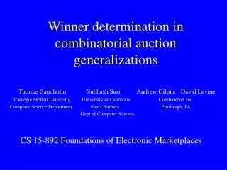
Winner determination in combinatorial auctions and generalizations. Andrew Gilpin 10/23/07. Solving the winner determination problem when all combinations can be bid on: Search algorithms for optimal anytime winner determination. Capitalize on sparsely populated space of bids

E N D
Winner determination in combinatorial auctions and generalizations Andrew Gilpin 10/23/07
Solving the winner determination problem when all combinations can be bid on:Search algorithms for optimal anytime winner determination • Capitalize on sparsely populated space of bids • Generate only populated parts of space of allocations • Highly optimized • 1st generation algorithm: branch-on-items formulation [Sandholm ICE-98, IJCAI-99, AIJ-02; Fujishima, Leyton-Brown & Shoham IJCAI-99] • 2nd generation algorithm: branch-on-bids formulation [Sandholm&Suri AAAI-00, AIJ-03, Sandholm et al. IJCAI-01] • New ideas, e.g., multivariate branching
Bids: 1 2 1 1,2 1,3,5 1,4 3 4 5 2 3 2 3,5 2,5 2,5 2 1,2 1,3,5 1,4 4 4 4 3 3,5 3 3 3,5 3 2,5 3,5 5 5 4 4 4 5 First generation search algorithms: branch-on-items formulation [Sandholm ICE-98, IJCAI-99, AIJ-02]
B A Bid graph A D C IN OUT B C B D C C OUT IN IN OUT C D C OUT IN D D IN OUT 2nd generation algorithm: Combinatorial Auction, Branch On Bids[Sandholm&Suri AAAI-00, AIJ-03] Bids of this example A={1,2} B={2,3} C={3} D={1,3} • Finds an optimal solution • Naïve analysis: 2#bids leaves • Thrm. At most leaves • where k is the minimum #items per bid • provably polynomial in bids even in worst case!
Use of h-values (=upper bounds) to prune winner determination search • f* = value of best solution found so far • g = sum of prices of bids that are IN on path • h = value of LP relaxation of remaining problem • Upper bounding: Prune the path when g+h ≤ f*
Linear program of the winner determination problem aka shadow price
Linear programming Original problem maximize such that Initial tableau Slack variables Assume, for simplicity, that origin is feasible (otherwise have to run a different LP to find first feasible and run the main LP in a revised space). Simplex method “pivots” variables in and out of the tableau Basic variables are on the left hand side
Graphical interpretation of simplex algorithm for linear programming Entering variable x1 x2 Departing variable Departing variable is slack variable of the constraint Constraints c Feasible region Each pivot results in a new tableau Entering variable x2 x1
Speeding up the use of linear programs in search • If LP returns a solution where all integer variables have integer values, then that is the solution to that node and no further search is needed below that node • Instead of simplex in the LP, use simplex in the DUAL because after branching, the previous DUAL solution is still feasible and a good starting point for simplex at the new node • Thrm. LP optimum value = DUAL optimum value aka shadow price
Cutting planes (aka cuts) • Extra linear constraints can be added to the LP to reduce the LP polytope and thus give tighter bounds (less optimistic h-values) if the constraints are guaranteed to not exclude any integer solutions • Applications-specific vs. general-purpose cuts • Branch-and-cut algorithm = branch-and-bound algorithm that uses cuts • A global cut is valid throughout the search tree • A local cut is guaranteed to be valid only in the subtree below the node at which it was generated (and thus needs to be removed from consideration when not in that subtree)
Example of a cut that is valid for winner determination: Odd hole inequality E.g., 5-hole x8 x3 x2 No chord x1 x6 Edge means that bids share items, so both bids cannot be accepted x1 + x2 + x3 + x6 + x8 ≤ 2
Valid cut that separates Valid cut that does not separate Invalid cut Separation using cuts LP optimum
How to find cuts that separate? • For some cut families (and/or some problems), there are polynomial-time algorithms for finding a separating cut • Otherwise, use: • Generate a cut • Generation preferably biased towards cuts that are likely to separate • Test whether it separates
Gomory mixed integer cut • Powerful general-purpose cut • Applicable to all problems, where • constraints and objective are linear, • the problem has integer variables and potentially also real variables • Cut is generated using the LP optimum so that the cut separates Curiosity: the problem could be solved with no search by an algorithm that generates a finite (potentially exponential) number of these cuts.
Not a slack variable LHS and RHS differ by an integer Derivation of Gomory mixed integer cut Input: optimal tableau row Define: non-basic, integer, continuous Rewrite tableau row: All integer terms add up to integers:
Structural improvements to search algorithms for winner determinationOptimum reached faster & better anytime performance • Always branch on a bid j that maximizes e.g. pj / |Sj| (presort) • Lower bounding: If g+L>f*, then f*g+L • Identify decomposition of bid graph in O(|E|+|V|) time & exploit • Pruning across subproblems (upper & lower bounding) by using f* values of solved subproblems and h values of yet unsolved ones • Forcing decomposition by branching on an articulation bid • All articulation bids can be identified in O(|E|+|V|) time • Could try to identify combinations of bids that articulate (cutsets)
Question ordering heuristics • In depth-first branch-and-bound, it is best to branch on a question for which the algorithm knows a good answer with high likelihood • Best (to date) heuristics for branching on bids[Sandholm,Suri,Gilpin&Levine IJCAI-01]: • A: Branch on bid whose LP value is closest to 1 • B: Branch on bid with highest normalized shadow surplus: • Choosing the heuristic dynamically based on remaining subproblem • E.g. use A when LP table density > 0.25 and B otherwise • In A* search, it is best to branch on a question whose right answer the algorithm is very uncertain about • Traditionally in OR, variable whose LP value is most fractional • More general idea [Gilpin&Sandholm 07]: branch on a question that reduces the entropy of the LP solution the most • Determine this e.g. based on lookahead • Applies to multivariate branching too
Identifying & solving tractable cases at search nodes(so that no search is needed below such nodes) [Sandholm & Suri AAAI-00, AIJ-03]
Example 1: “Short” bids [Sandholm&Suri AAAI-00, AIJ-03] • Never branch on short bids with 1 or 2 items • At each search node, we solve short bids from bid graph separately • O(#short bids 3) time using maximal weighted matching • [Edmonds 65; Rothkopf et al 98] • NP-complete even if only 3 items per bid allowed • Dynamically delete items included in only one bid
Example 2: Interval bids • At each search node, use a polynomial algorithm if remaining bid graph only contains interval bids • Ordered list of items: 1..#items • Each bid is for some interval [q, r] of these items • [Rothkopf et al. 98] presented O(#items2) DP algorithm • [Sandholm&Suri AAAI-00, AIJ-03] DP algorithm is O(#items + #bids) • Bucket sort bids in ascending order of r • opt(i) is the optimal solution using items 1..i • opt(i) = max b in bids whose last item is i {pb + opt(qb-1), opt(i-1)} • Identifying linear ordering • Can be identified in O(|E|+|V|) time [Korte & Mohring SIAM-89] • Interval bids with wraparound can be identified in O(#bids2) time [Spinrad SODA-93] and solved in O(#items (#items + #bids)) time using our DP while DP of Rothkopf et al. is O(#items3)
Example 3: [Sandholm & Suri AAAI-00, AIJ-03]
Example 3... • Thrm. [Conitzer, Derryberry & Sandholm AAAI-04]An item tree that matches the remaining bids (if one exists) can be constructed in time O(|Bids| |#items that any one bid contains|2 + |Items|2) • Algorithm: • Make a graph with the items as vertices • Each edge (i, j) gets weight #(bids with both i and j) • Construct maximum spanning tree of this graph: O(|Items|2) time • Thrm. The resulting tree will have the maximum possible weight #(occurrences of items in bids) - |Bids| iff it is a valid item tree • Complexity of constructing an item graph of treewidth 2 (or 3, or 4, …) is unknown (but complexity of solving any such case given the item graph is “polynomial-time” - exponential only in the treewidth)
Preprocessors [Sandholm IJCAI-99, AIJ-02] • Only keep highest bid for each combination that has received bids • Superset pruning • E.g. {1,2,3,4}, $10 is pruned by {1,3}, $7 and {2,4}, $6 • For each bid (prunee), use same search algorithm as main search, except restrict to bids that are subsets of prunee • Terminate the search and prune the prunee if f* ≥ prunee’s price • Only consider bids with ≤ 30 items as potential prunees • Tuple pruning • E.g. {1,2}, $8 and {3,4}, $3 are not competitive together given {1,3}, $7 and {2,4}, $6 • Construct virtual prunee from pair of bids with disjoint item sets • Use same pruning algorithm as superset pruning • If pruned, insert an edge into bid graph between the bids • O(#bids2 cap #items) • O(#bids3 cap #items) for pruning triples, etc. • More complex checking required in main search
Other generalizations of combinatorial auctions[Sanholm, Suri, Gilpin & Levine IJCAI-01 workshop, AAMAS-02] • Free disposal vs. no free disposal • Single vs. multiple units of each item • Auction vs. reverse auction vs. exchange • Reservation prices
Combinatorial reverse auction • Example: procurement in supply chains • Auctioneer wants to buy a set of items (has to get all) • Can take extras if there is free disposal • Sellers place bids on how cheaply they are willing to sell bundles of items • Thrm. Winner determination is NP-complete even in single-unit case with free disposal • Thrm. Single unit case with free disposal is approximable • k = 1 + log m (m = largest number of items that any bid contains) • Greedy algorithm: Keep choosing bid with lowest price / #items
No free disposal • Free disposal: seller can keep items, buyers can take extras • Free disposal usually assumed in the combinatorial auction literature • In practice, freeness of disposal can vary across items & bidders • Without free disposal, the set of feasible solutions is same for combinatorial auctions & reverse auctions • Thrm. Without free disposal, even finding a feasible solution is NP-complete
Combinatorial exchange • Example bid: (buy 20 tons of water, sell 10 cubic meters of hydrogen, sell 5 cubic meters of oxygen, ask $500) • Example application: manufacturing where a participant bids for inputs & outputs of a production plan simultaneously • Label bids as winning or losing so as to maximize (revealed) surplus: sum of amounts paid by bidders minus sum of amounts paid to bidders • On each item, sell quantity buy quantity • Equality if there is no free disposal • Alternatively, could maximize liquidity (trading volume) • Thrm. NP-complete even in the single-unit case • Thrm. Inapproximable even in the single-unit case • Thrm. Without free disposal, even finding a feasible solution is NP-complete (even in the single-unit case)